Correlations

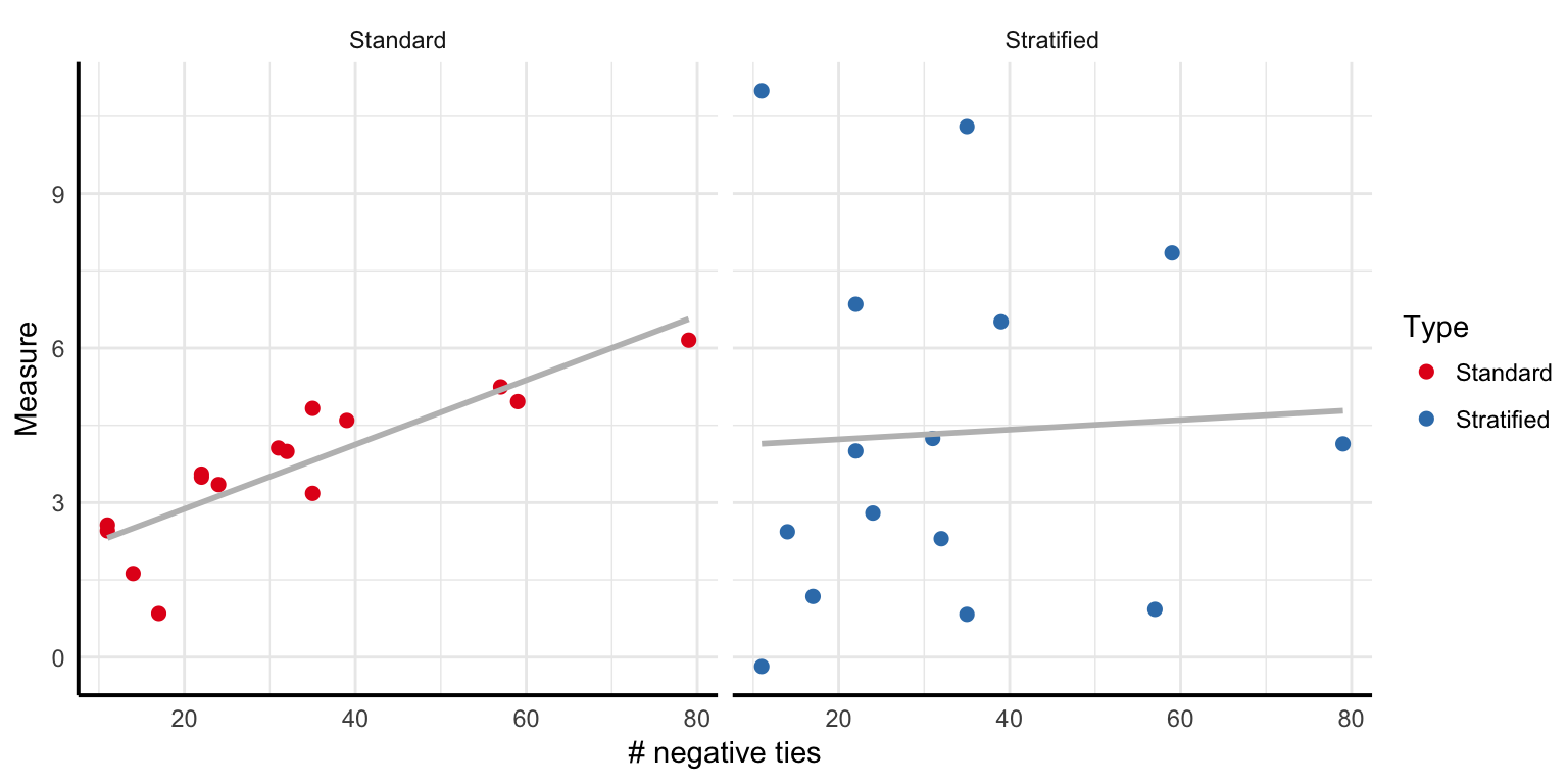
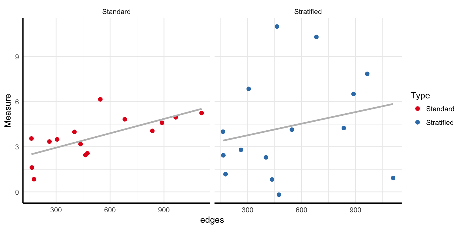
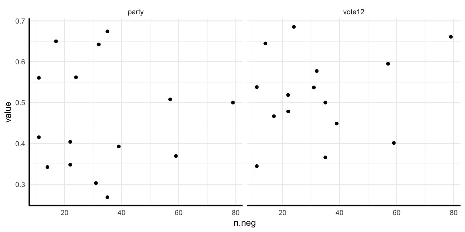
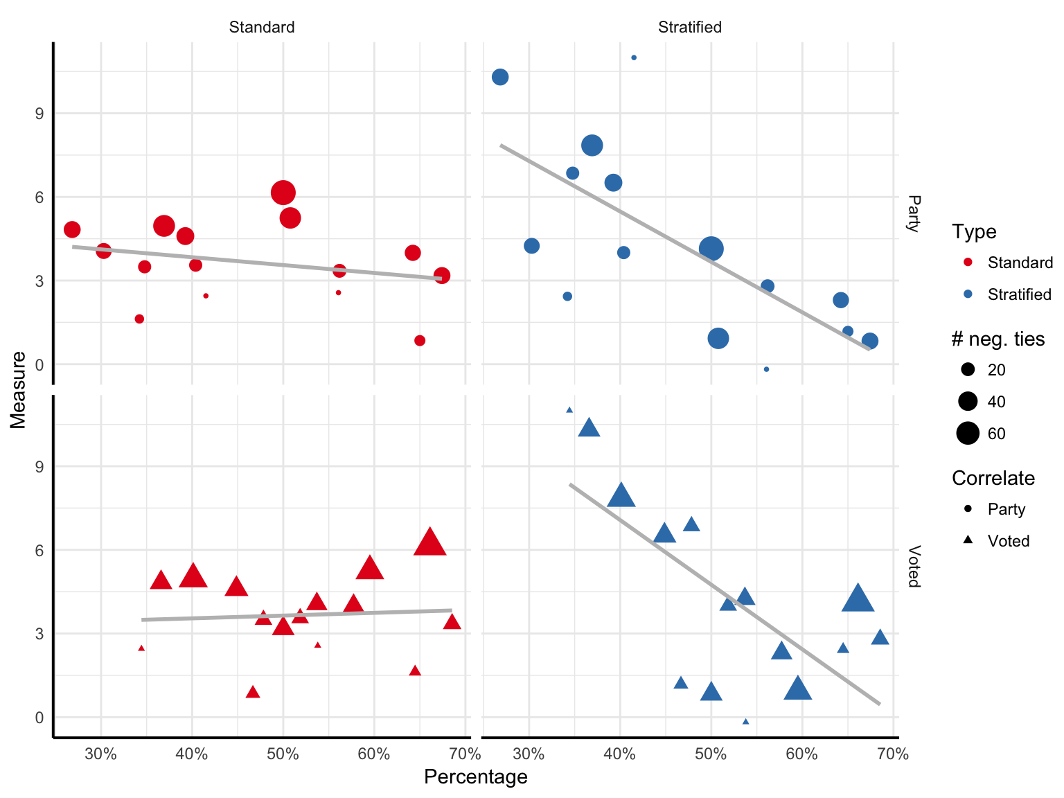
Looking into measure of balance vs. certain covariates, and comparing standard to stratified version.

Call:
lm(formula = strat.meas ~ party, data = all %>% filter(id != 
    24 & n.neg > 10))

Residuals:
    Min      1Q  Median      3Q     Max 
-4.0902 -2.0027  0.3126  1.0514  5.7934 

Coefficients:
            Estimate Std. Error t value Pr(>|t|)    
(Intercept)   12.711      2.516   5.052 0.000222 ***
party        -18.085      5.242  -3.450 0.004311 ** 
---
Signif. codes:  0 '***' 0.001 '**' 0.01 '*' 0.05 '.' 0.1 ' ' 1

Residual standard error: 2.597 on 13 degrees of freedom
Multiple R-squared:  0.4779,    Adjusted R-squared:  0.4378 
F-statistic:  11.9 on 1 and 13 DF,  p-value: 0.004311

Call:
lm(formula = stan.meas ~ party, data = all %>% filter(id != 24 & 
    n.neg > 10))

Residuals:
     Min       1Q   Median       3Q      Max 
-2.37613 -0.65420 -0.03081  0.78884  2.59940 

Coefficients:
            Estimate Std. Error t value Pr(>|t|)   
(Intercept)    4.965      1.372   3.619  0.00312 **
party         -2.821      2.859  -0.987  0.34174   
---
Signif. codes:  0 '***' 0.001 '**' 0.01 '*' 0.05 '.' 0.1 ' ' 1

Residual standard error: 1.416 on 13 degrees of freedom
Multiple R-squared:  0.06969,   Adjusted R-squared:  -0.001874 
F-statistic: 0.9738 on 1 and 13 DF,  p-value: 0.3417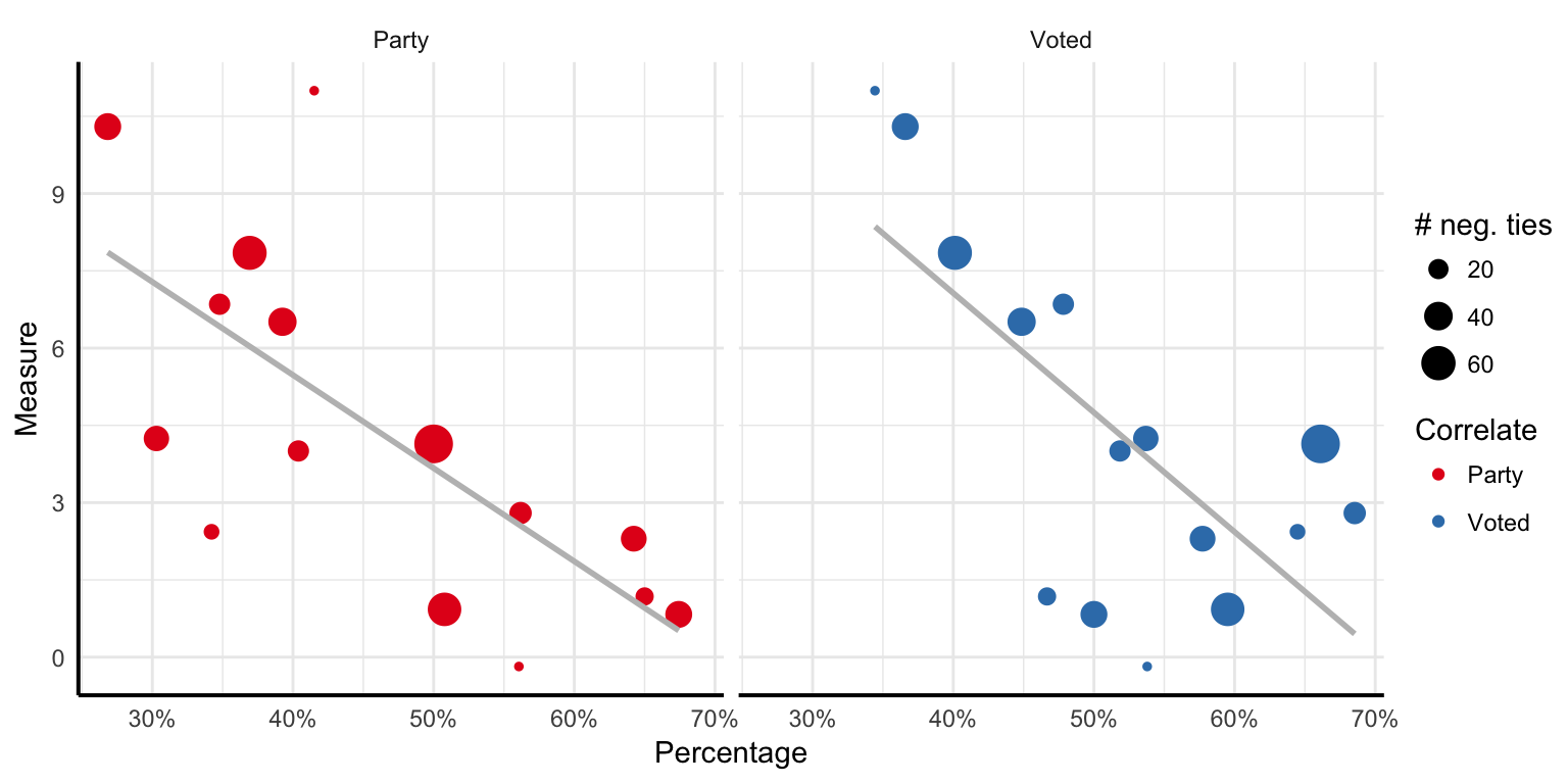

This plot essentially shows that the standard measure is simply correlating itself with the size of the graph.