Covariates

Graph Em All

After so many iterations, it’s probably time to redo the graphs, and see if they make sense.

1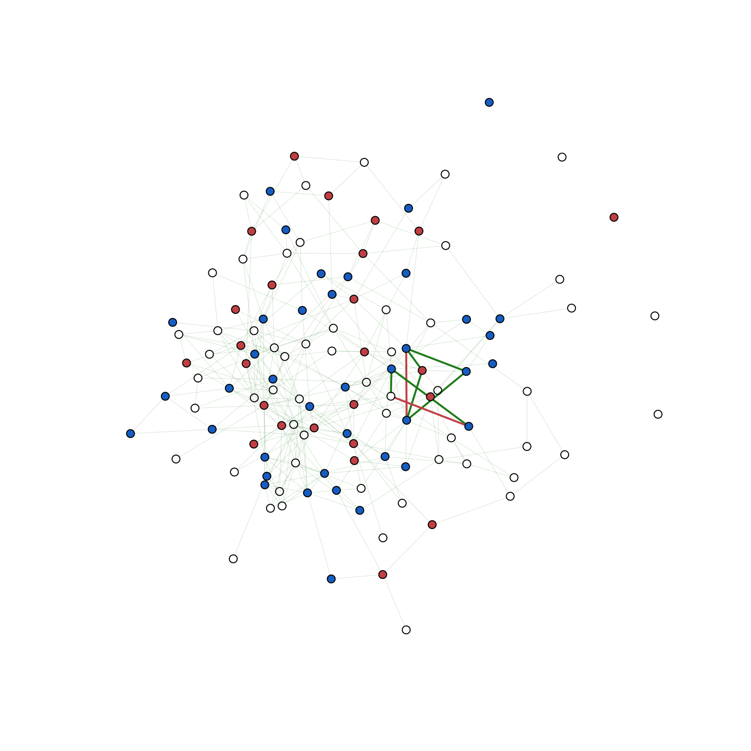

2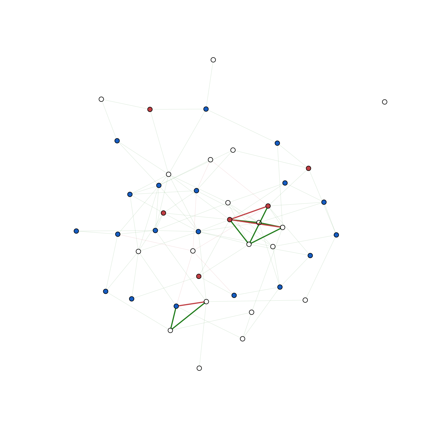

3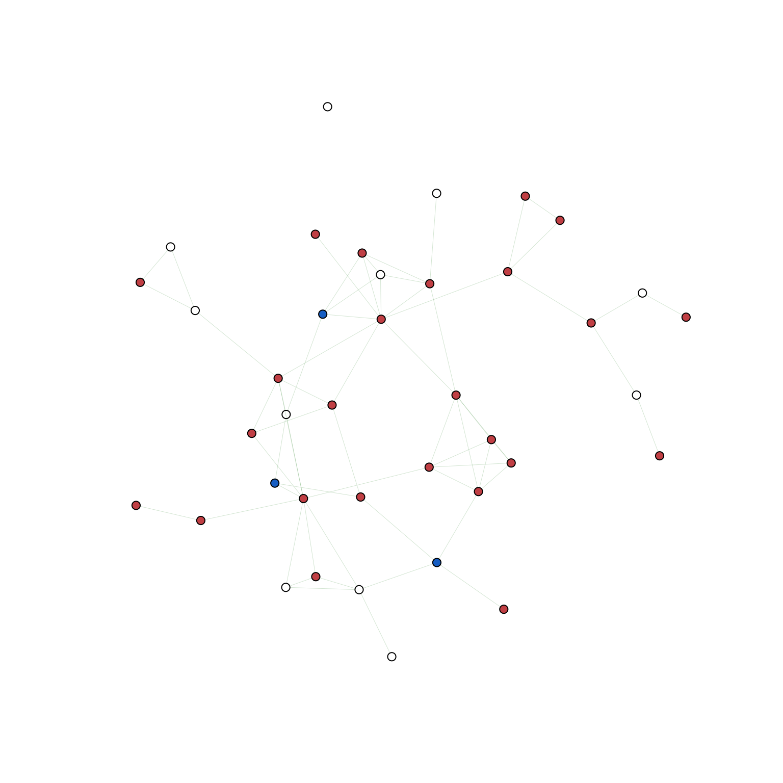

4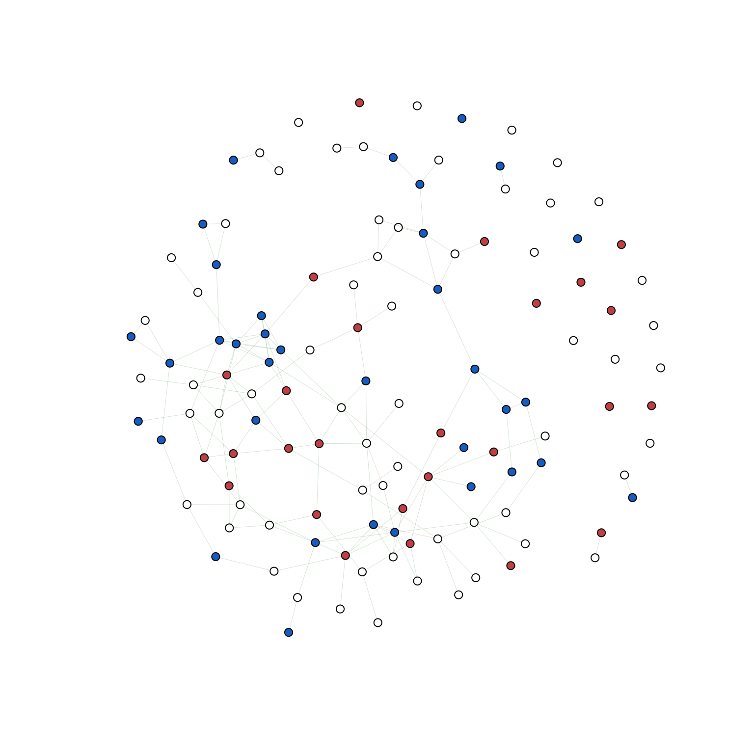

5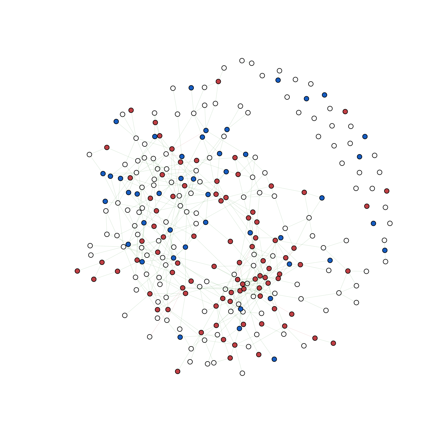

6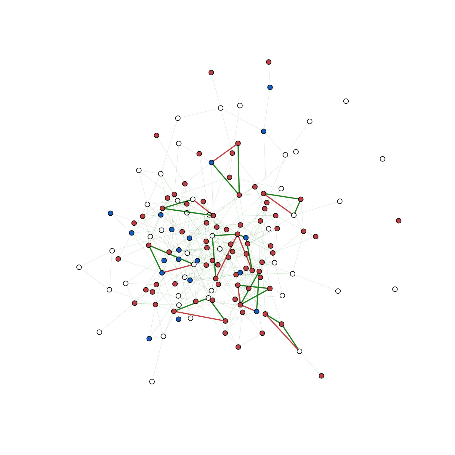

7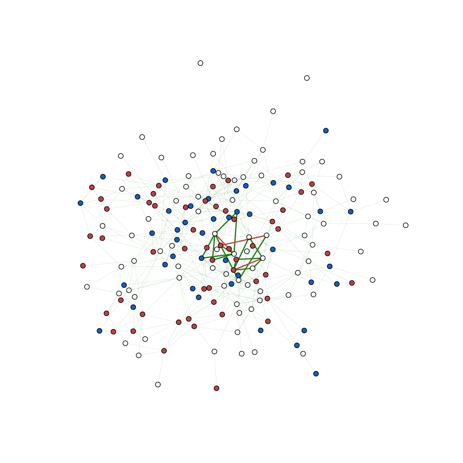

8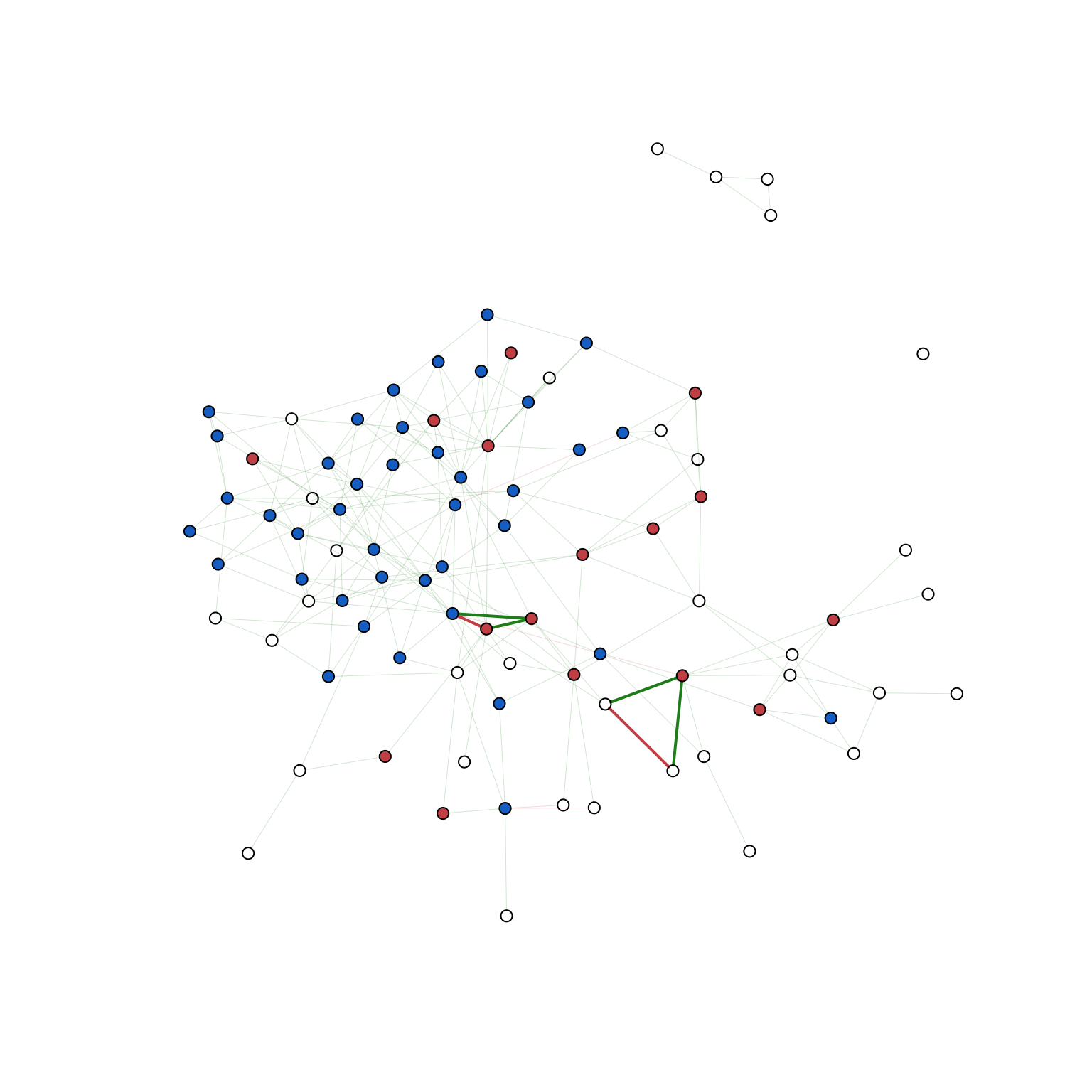

9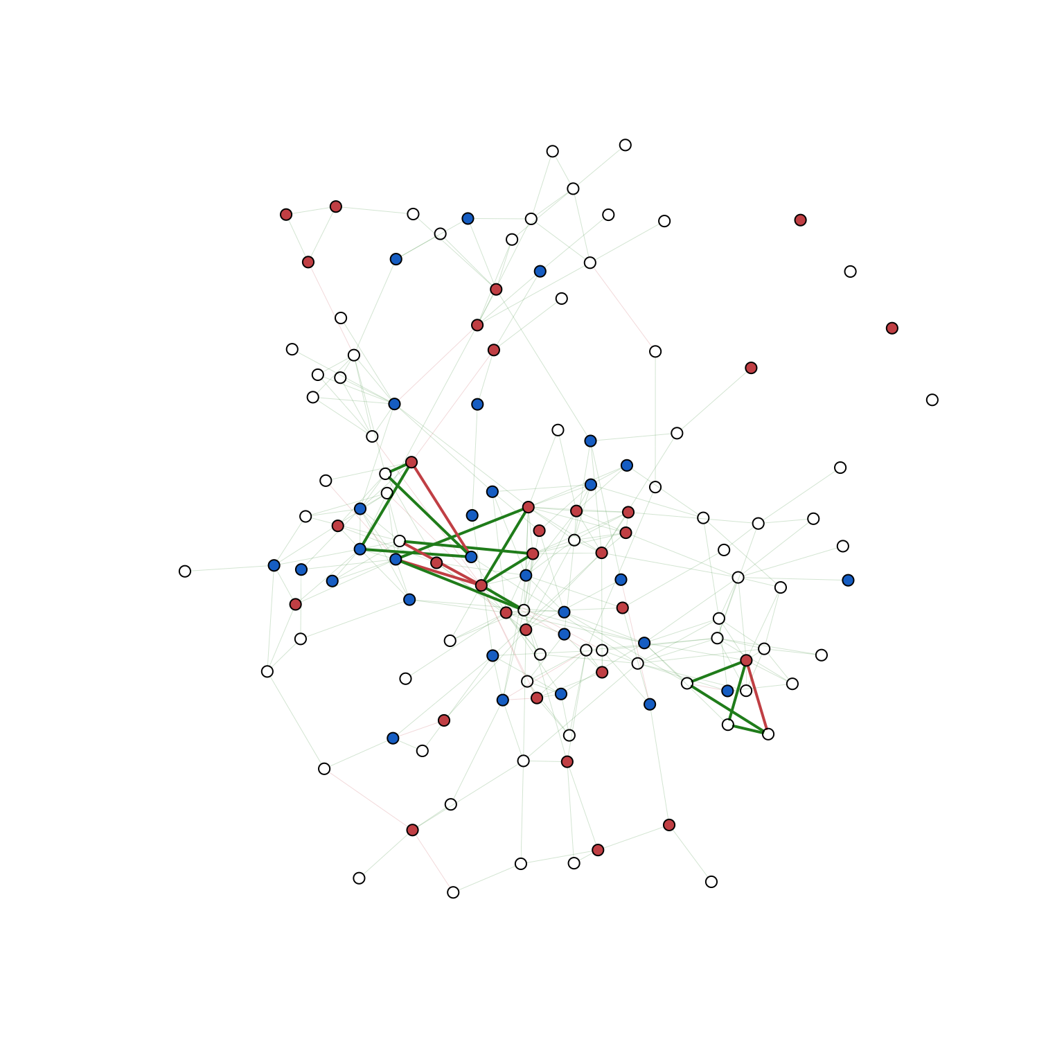

10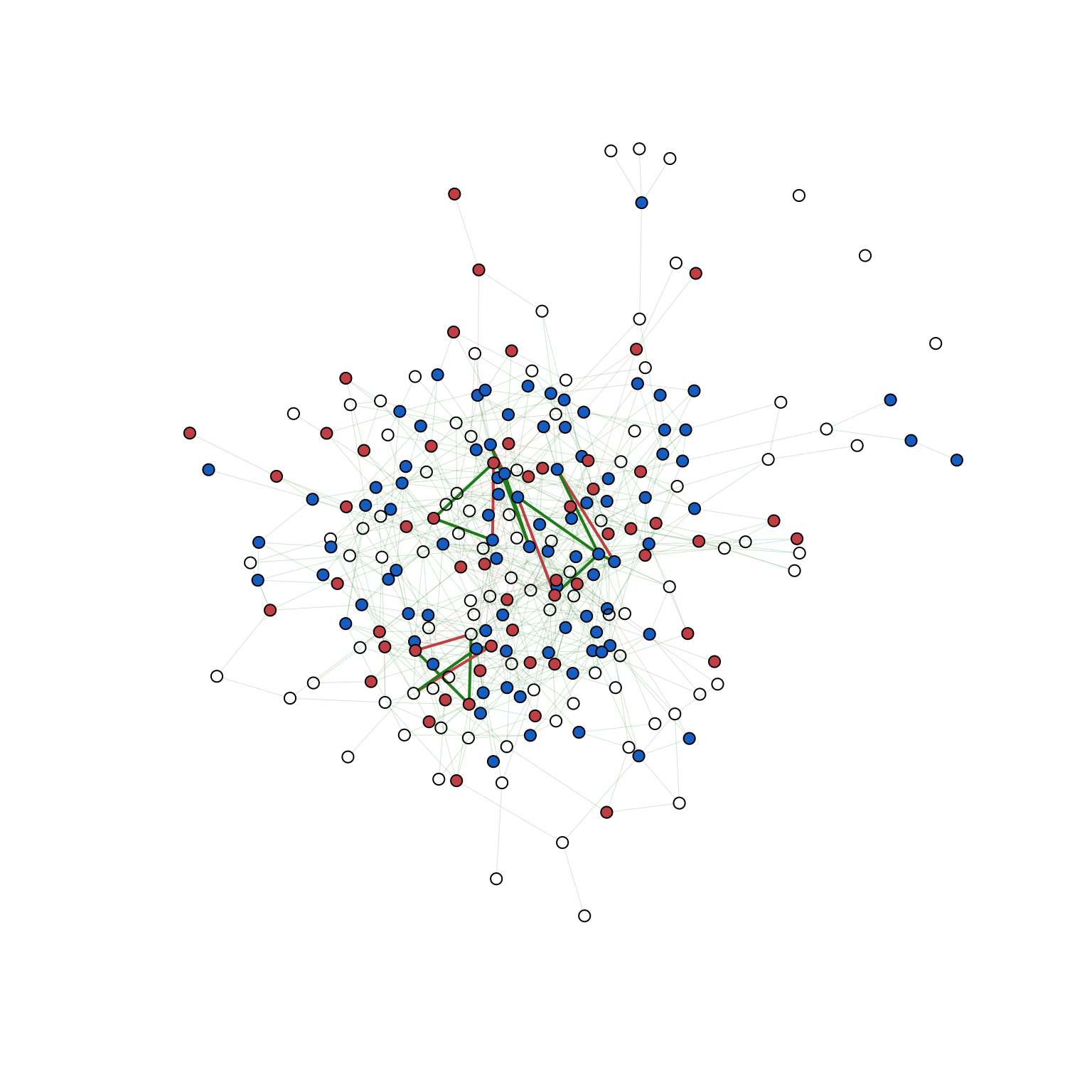

11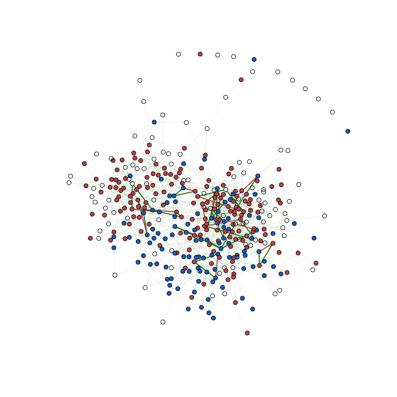

12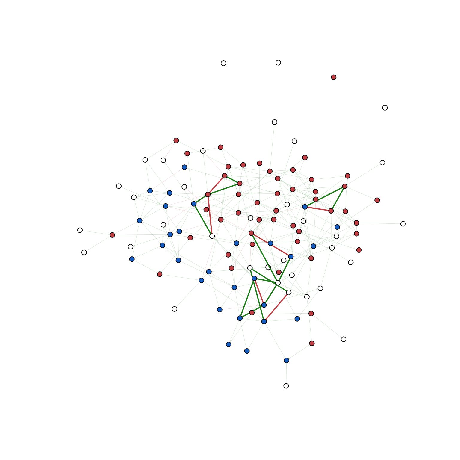

13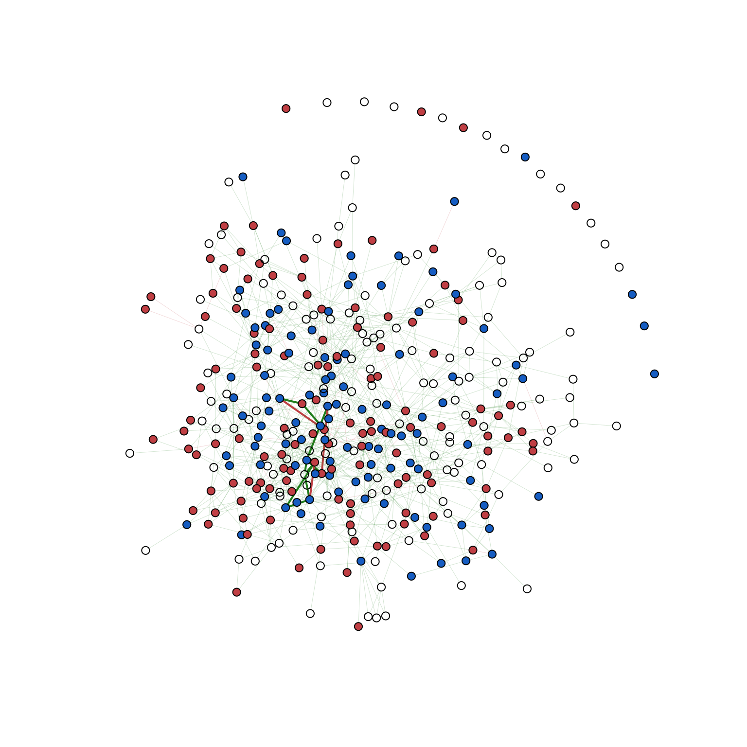

14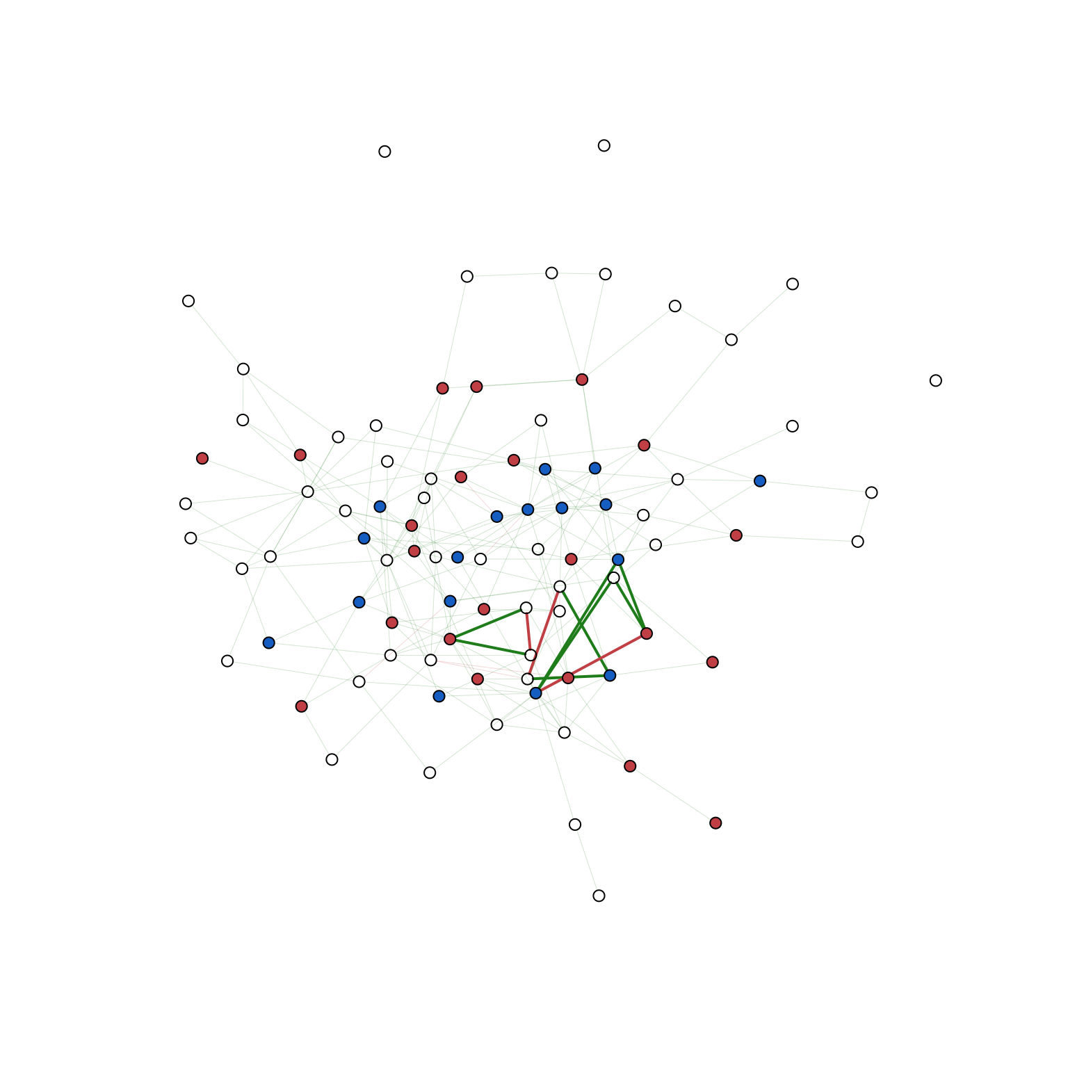

15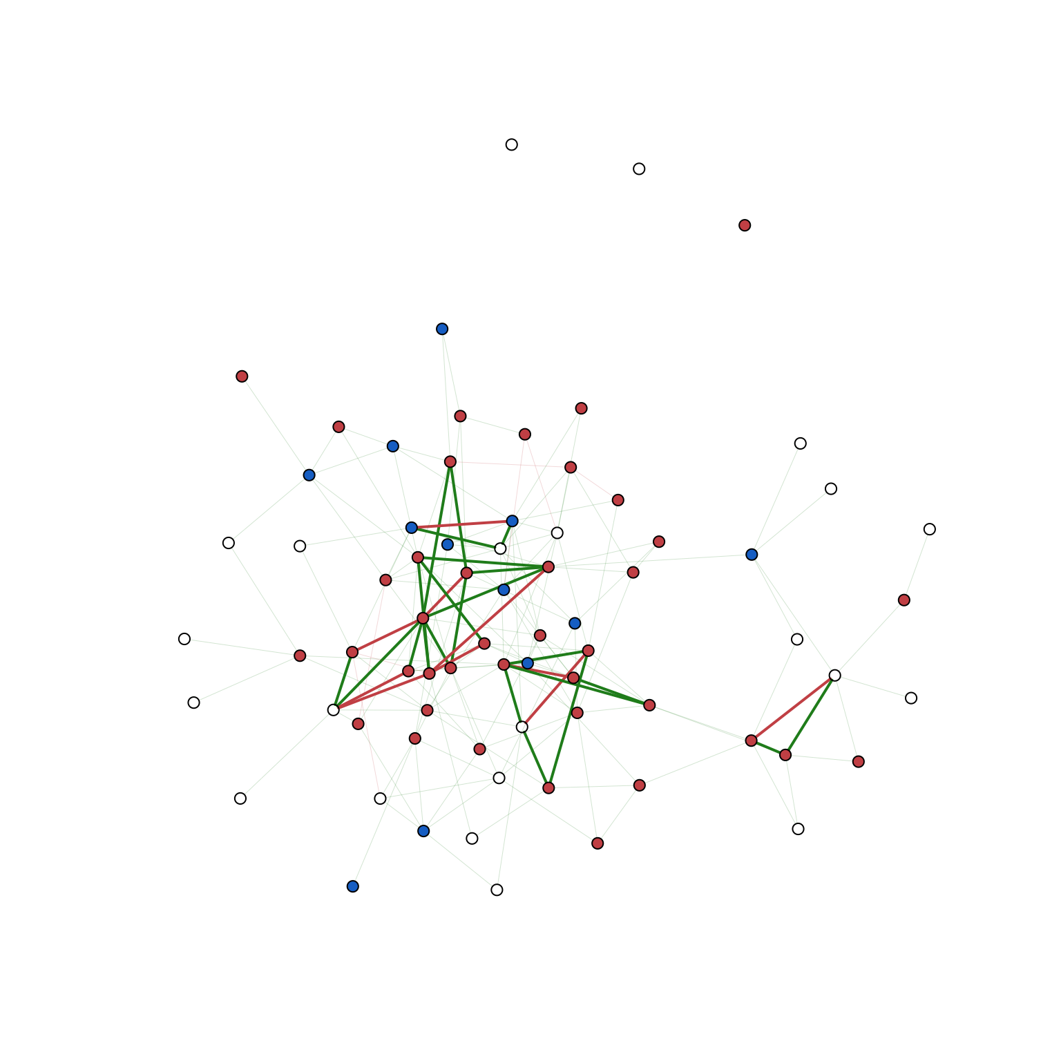

16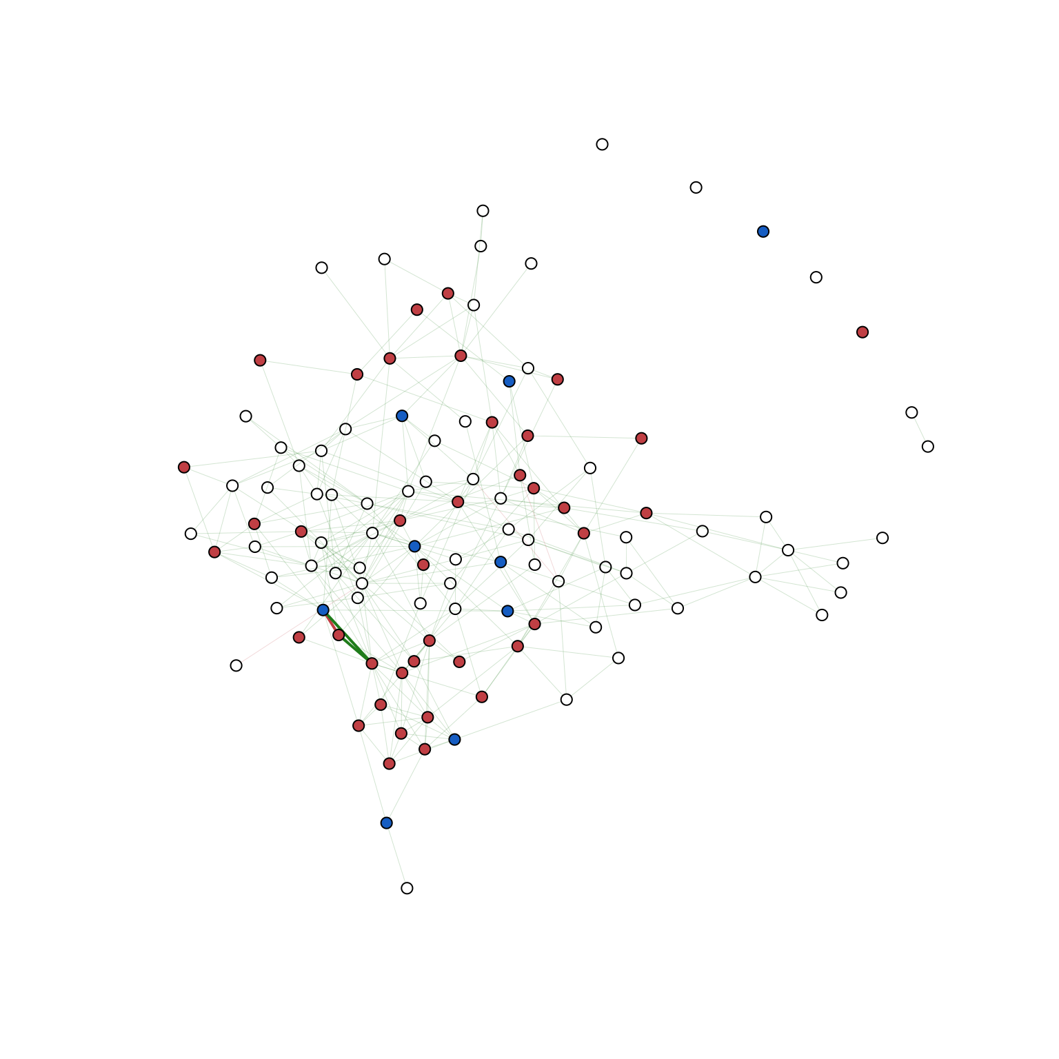

17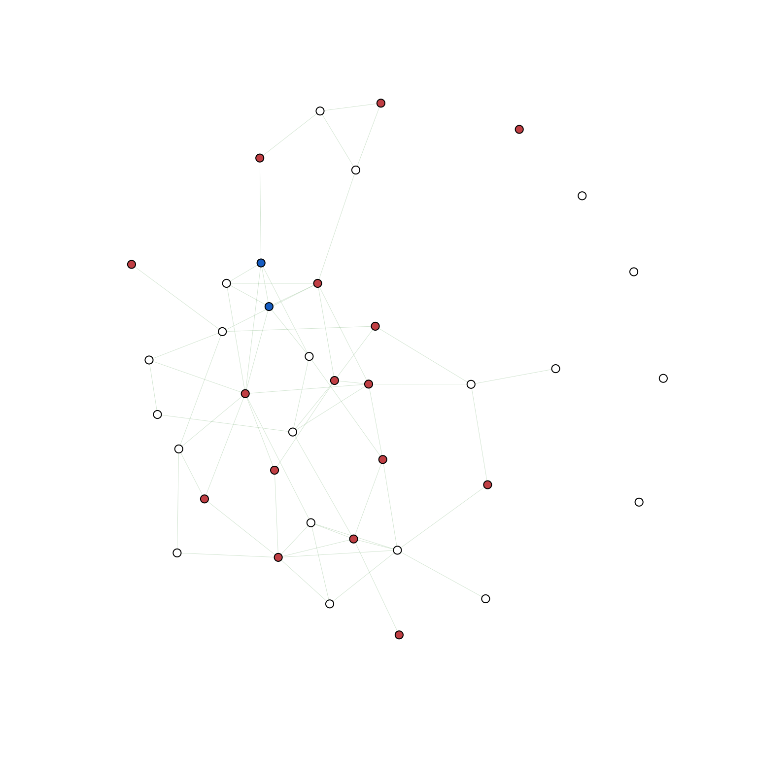

18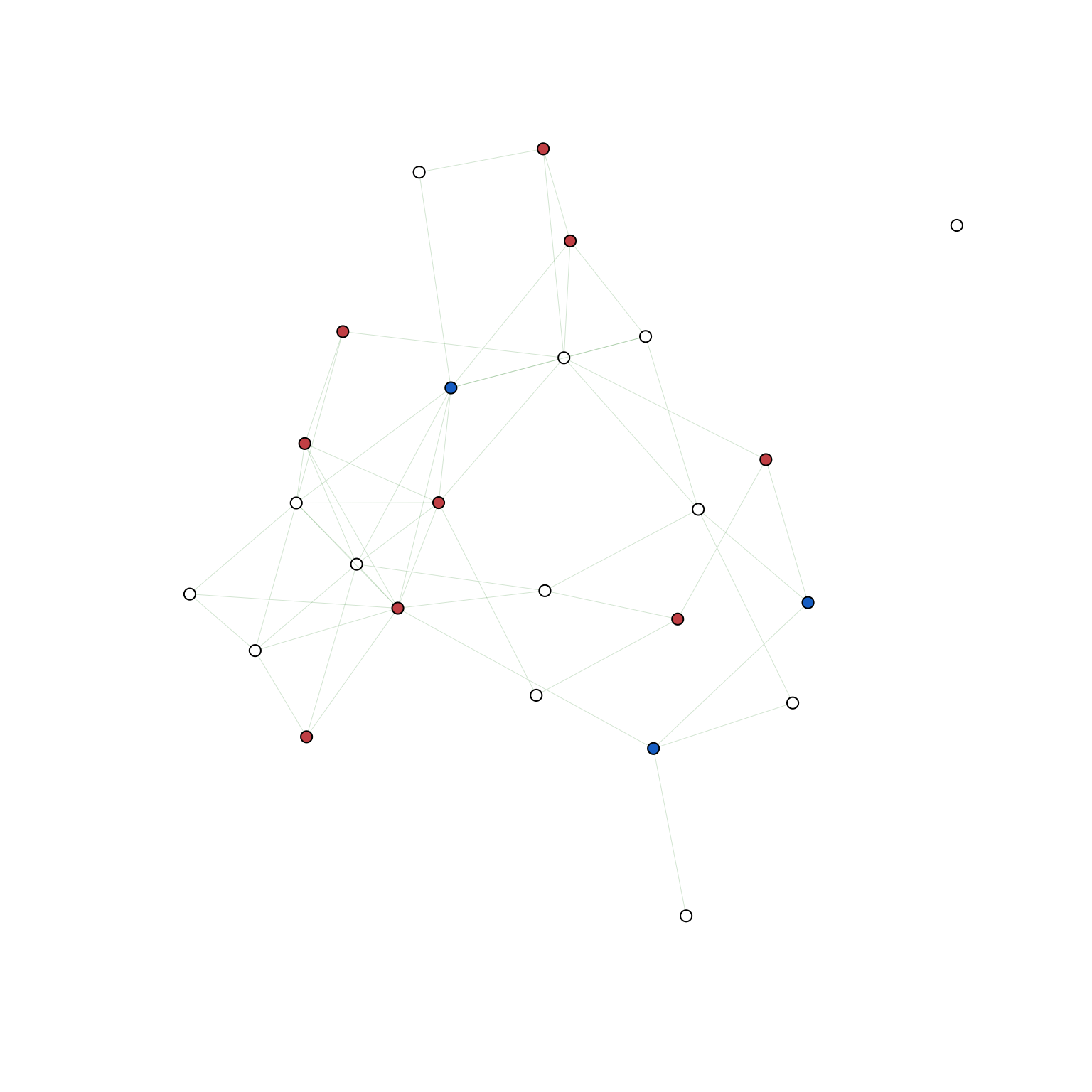

19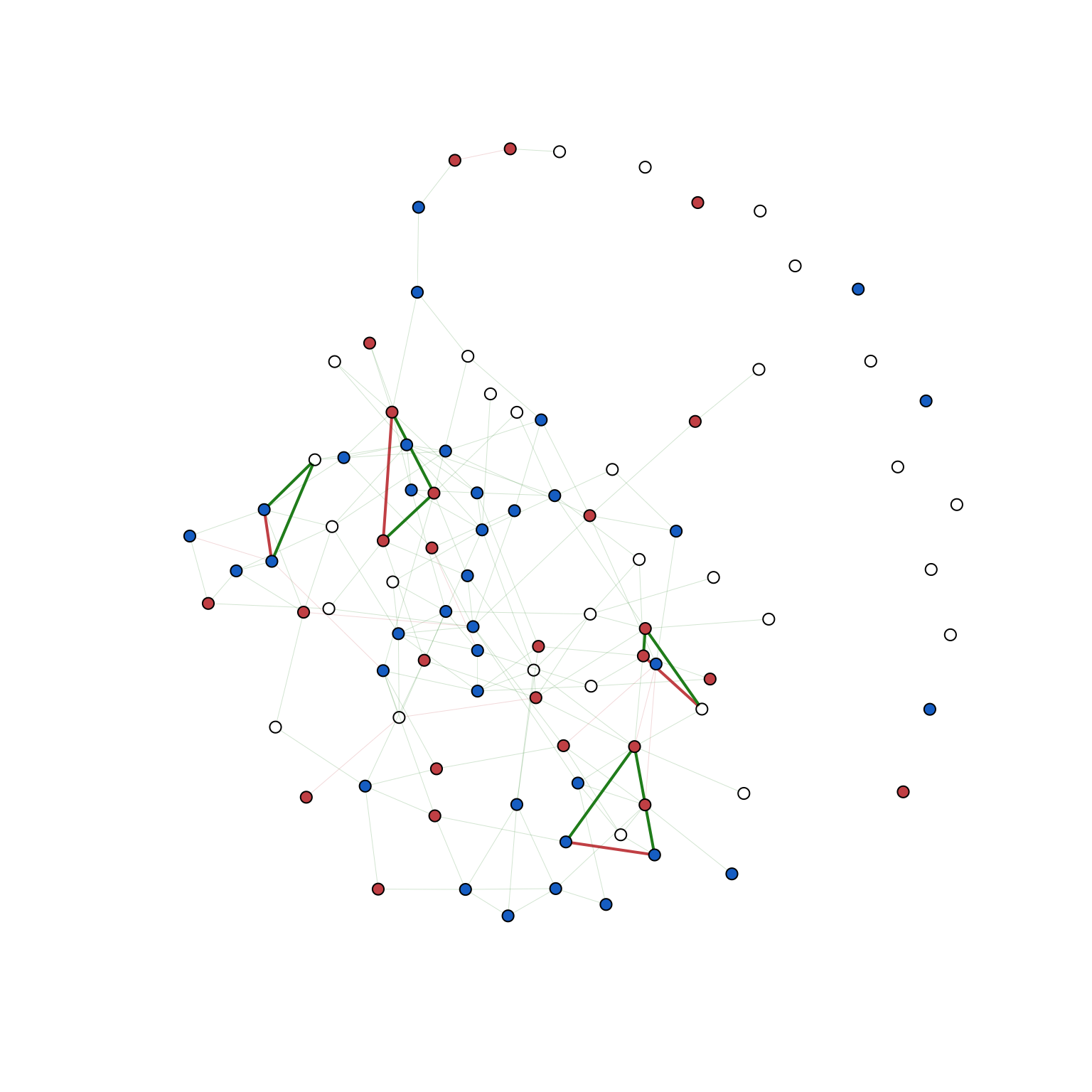

20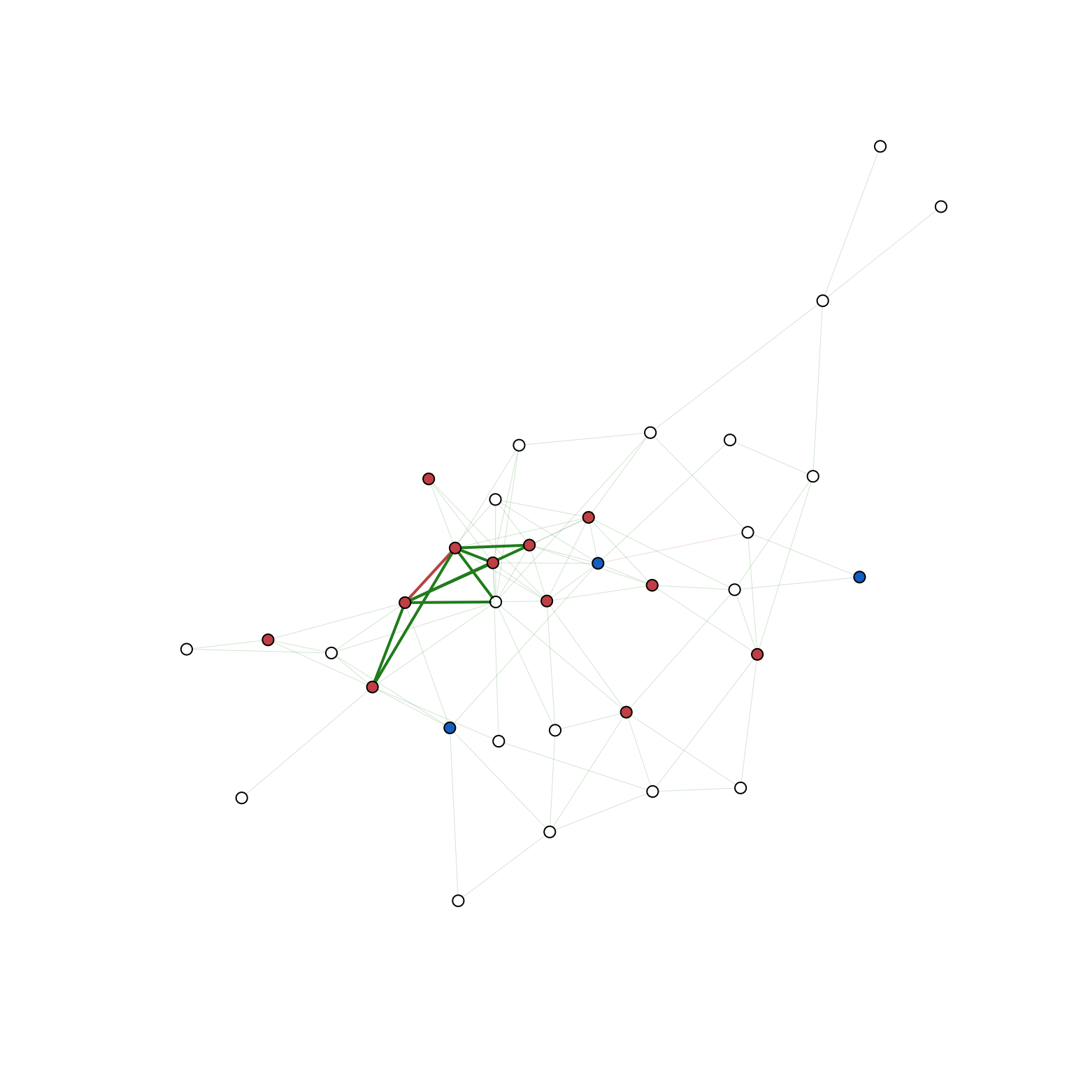

21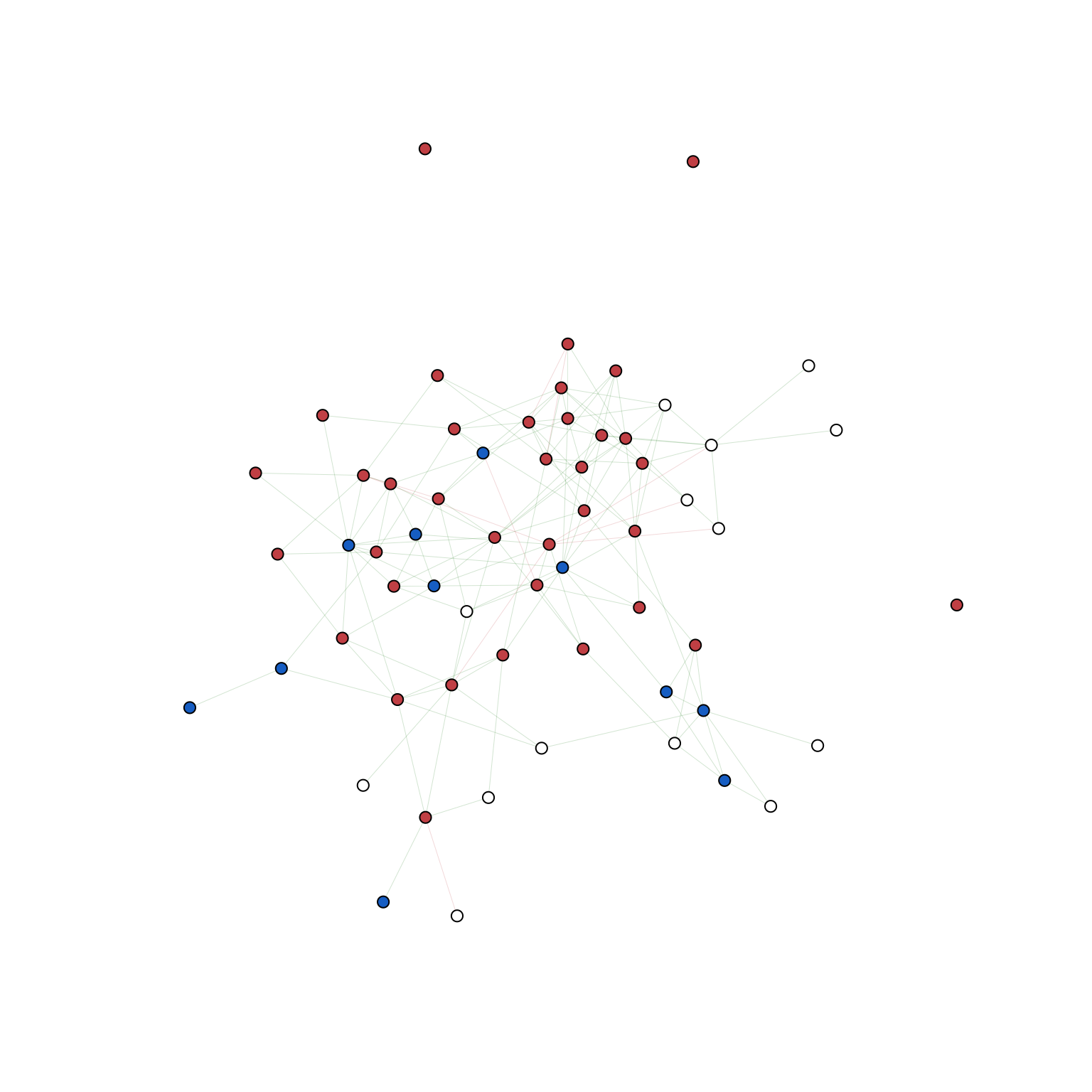

22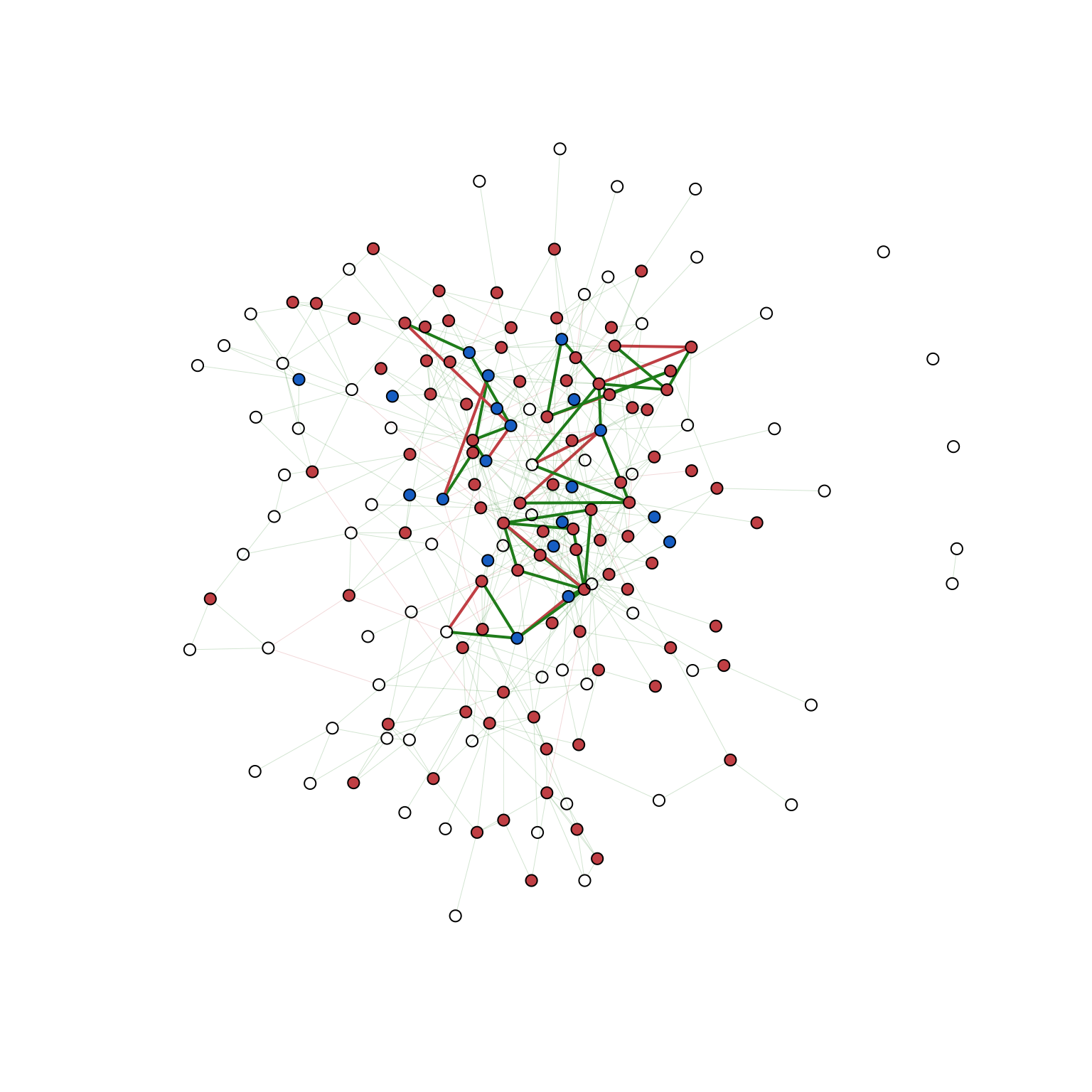

23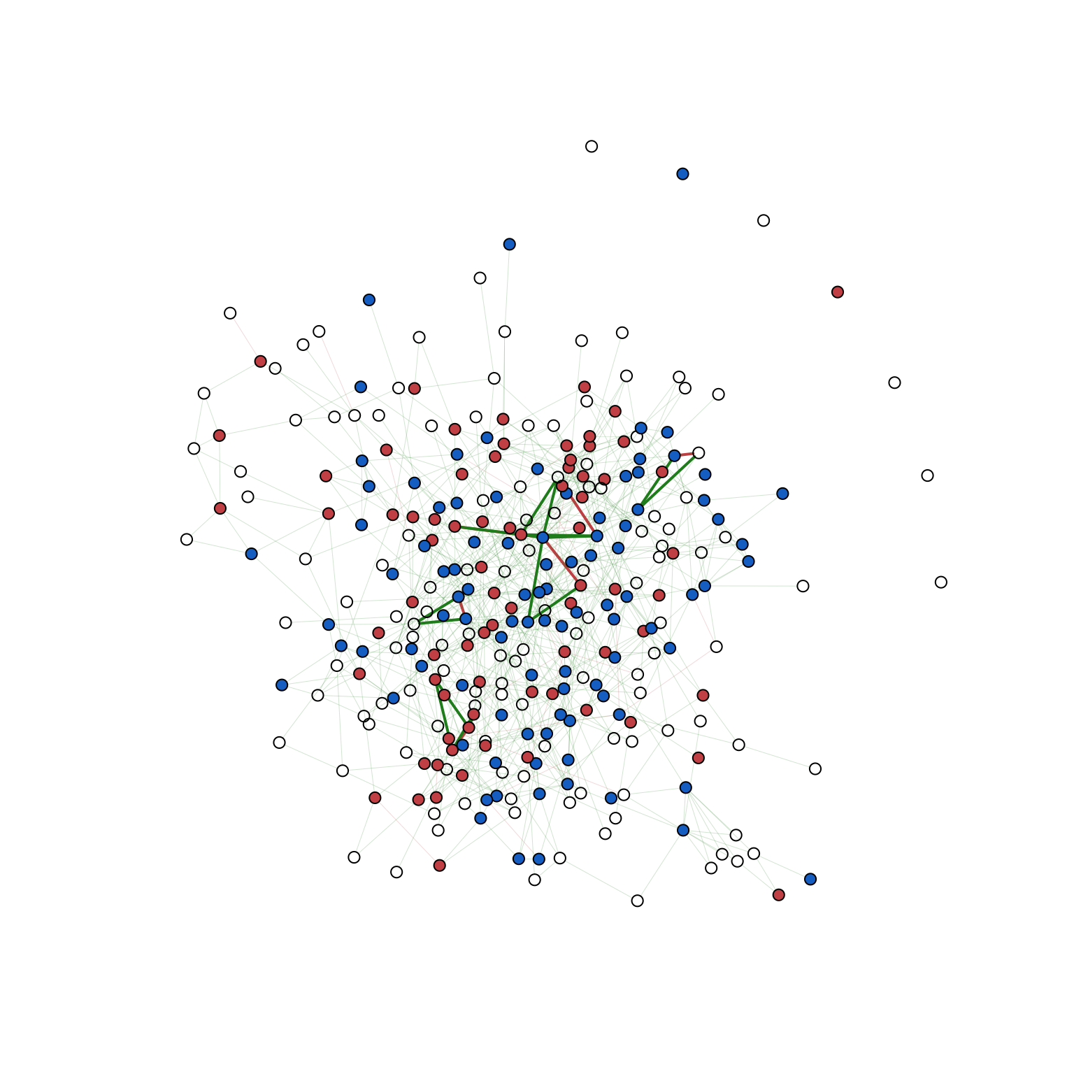

24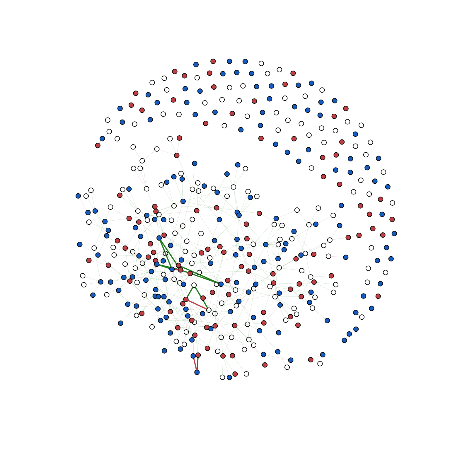

25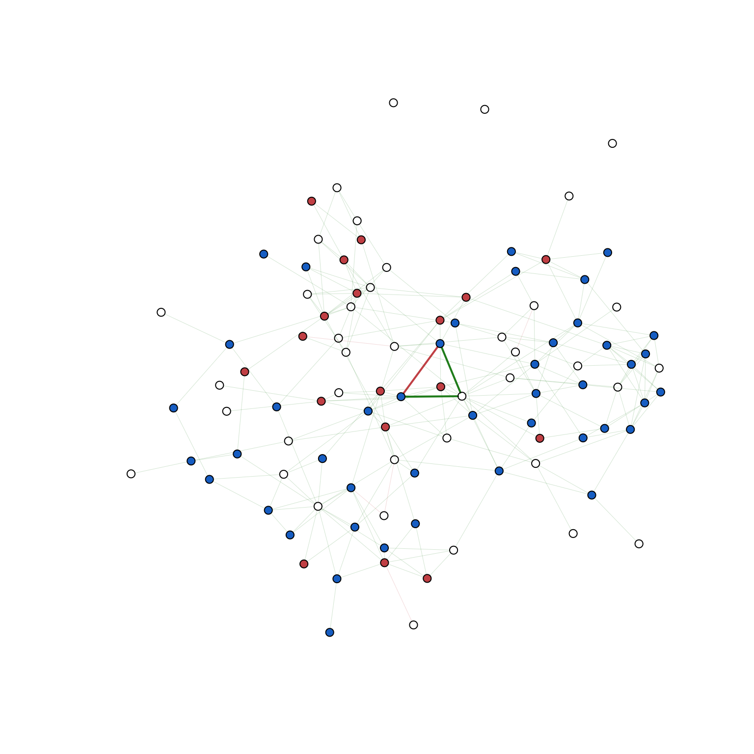

26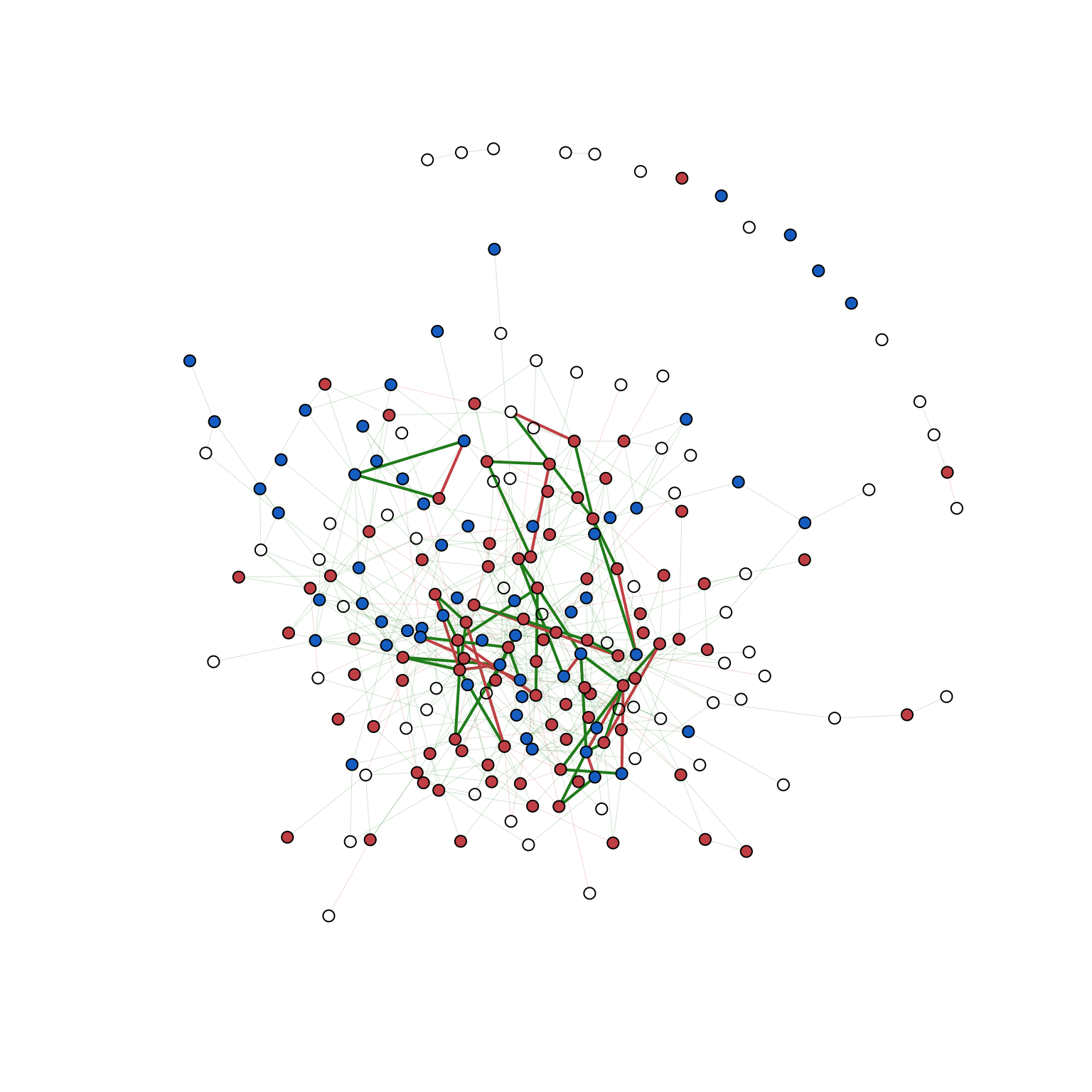

27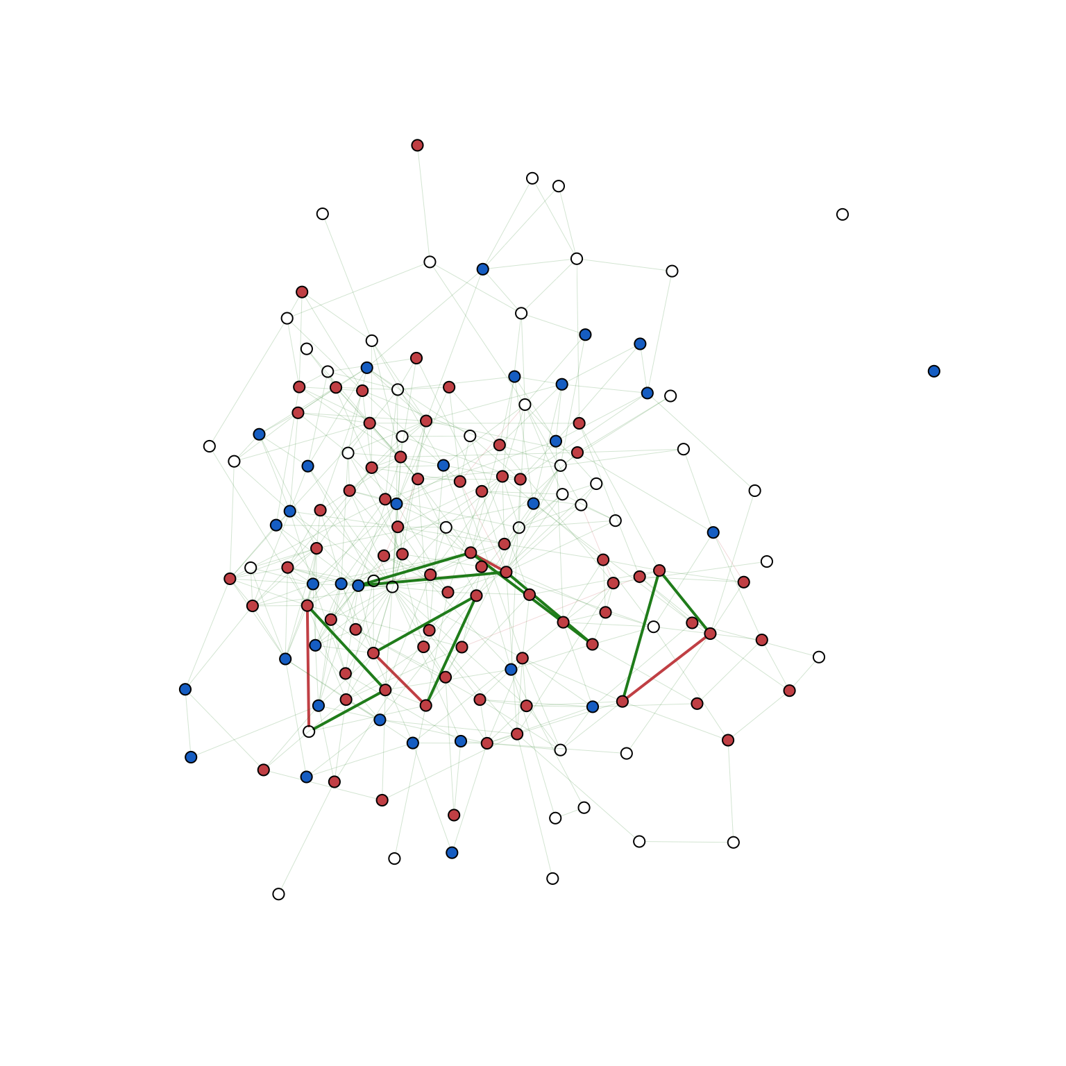

28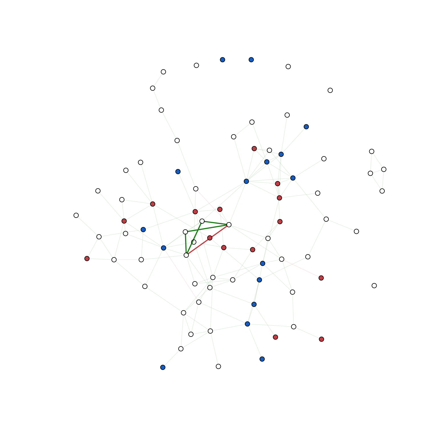

29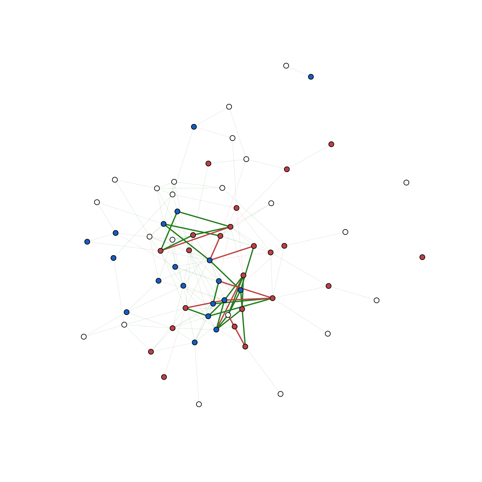

30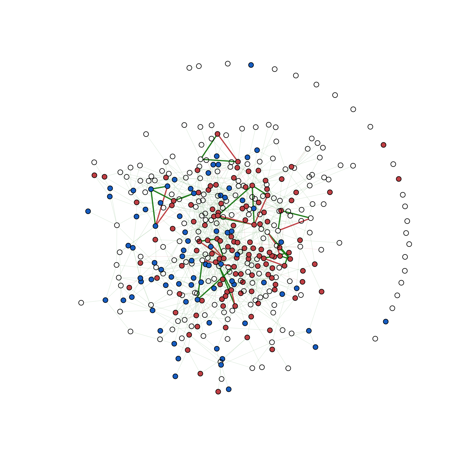

31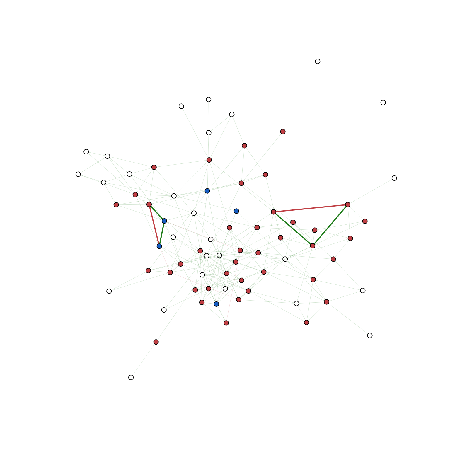

32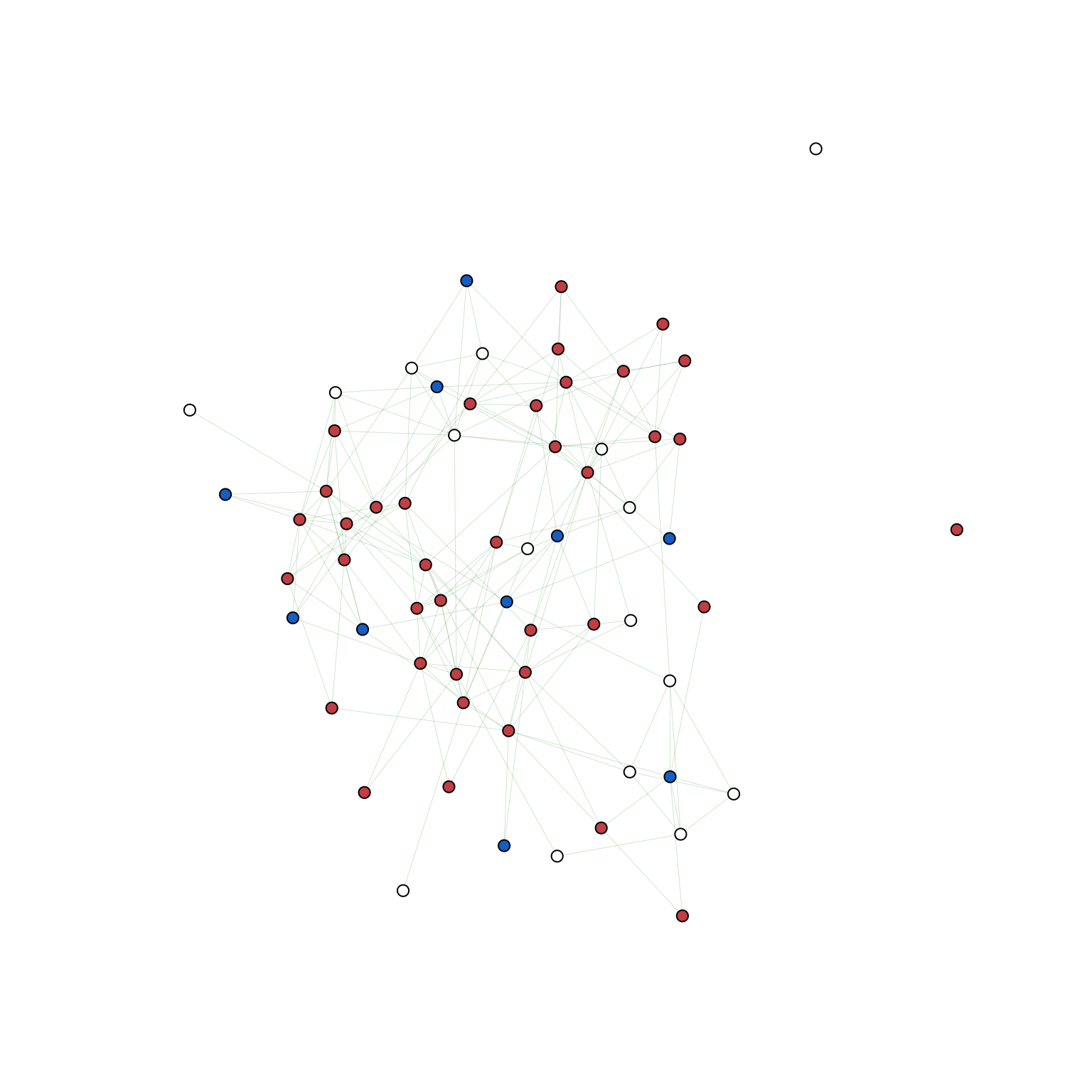

Subgraphs of Genders

1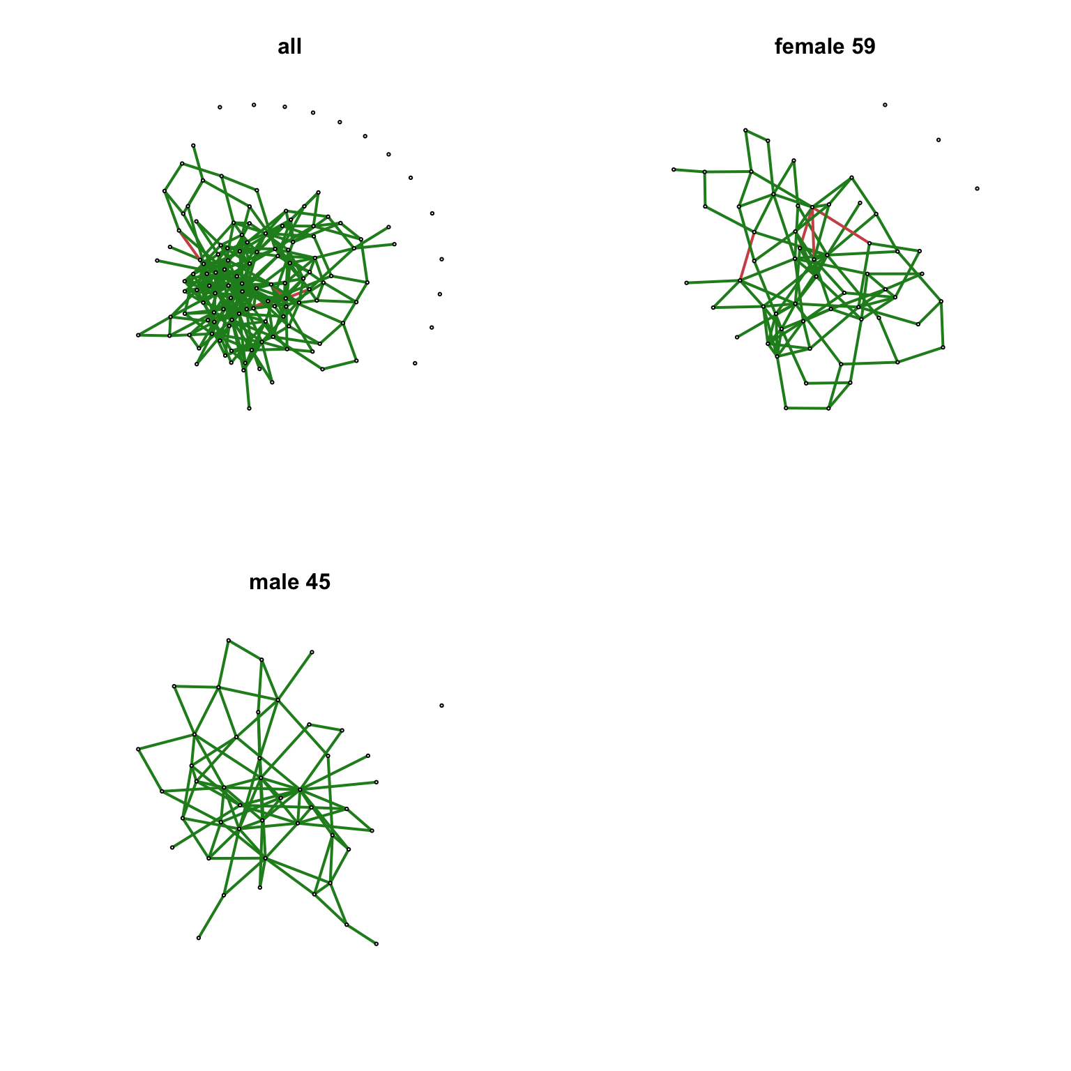

2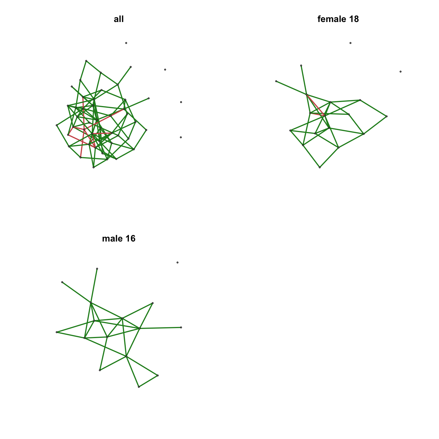

3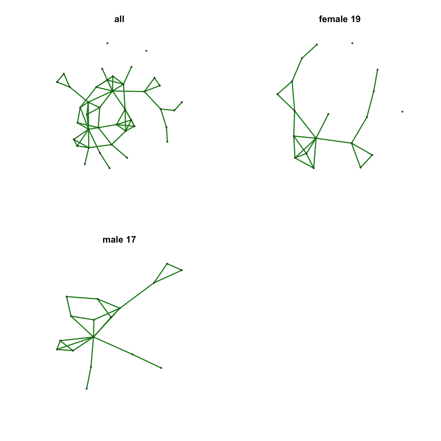

4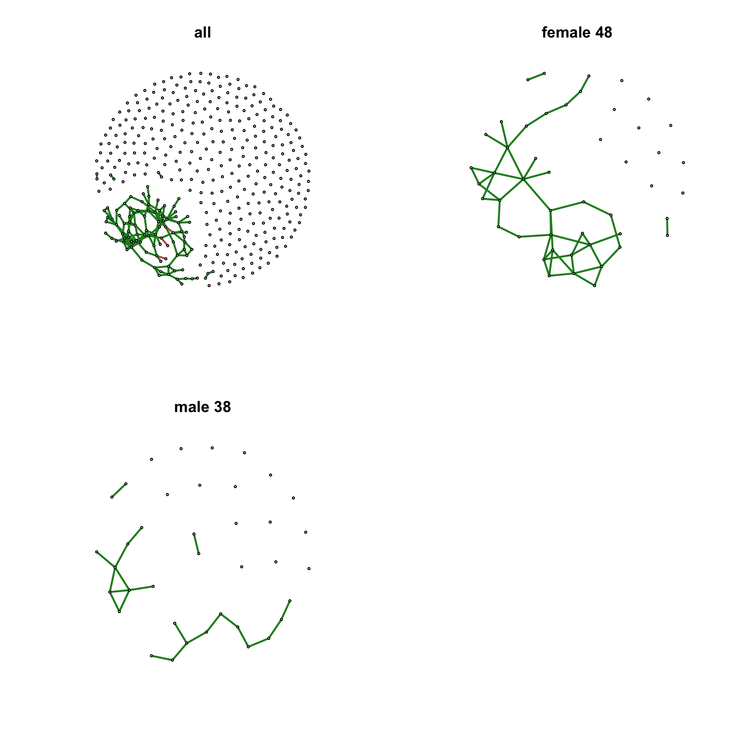

5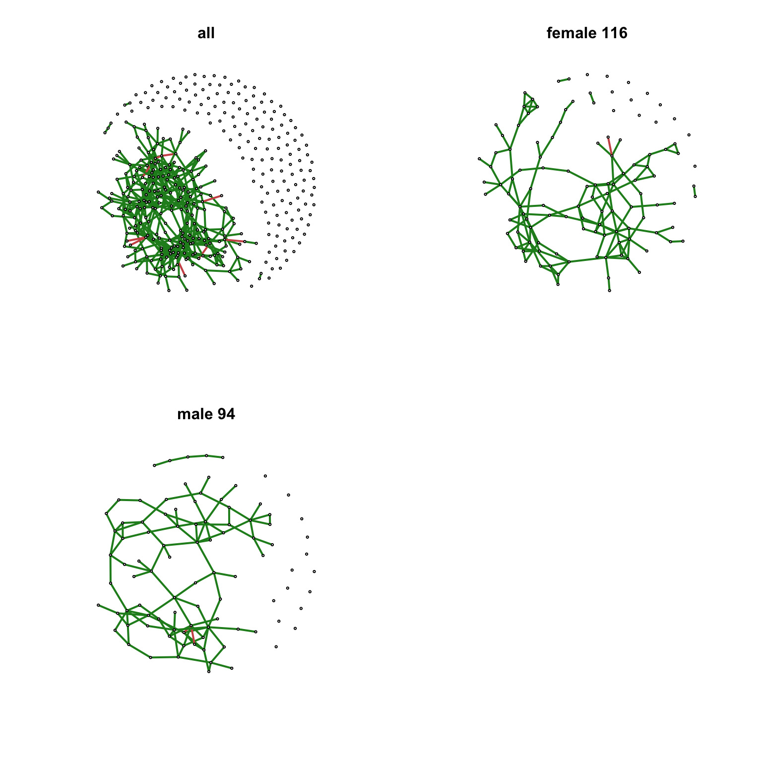

6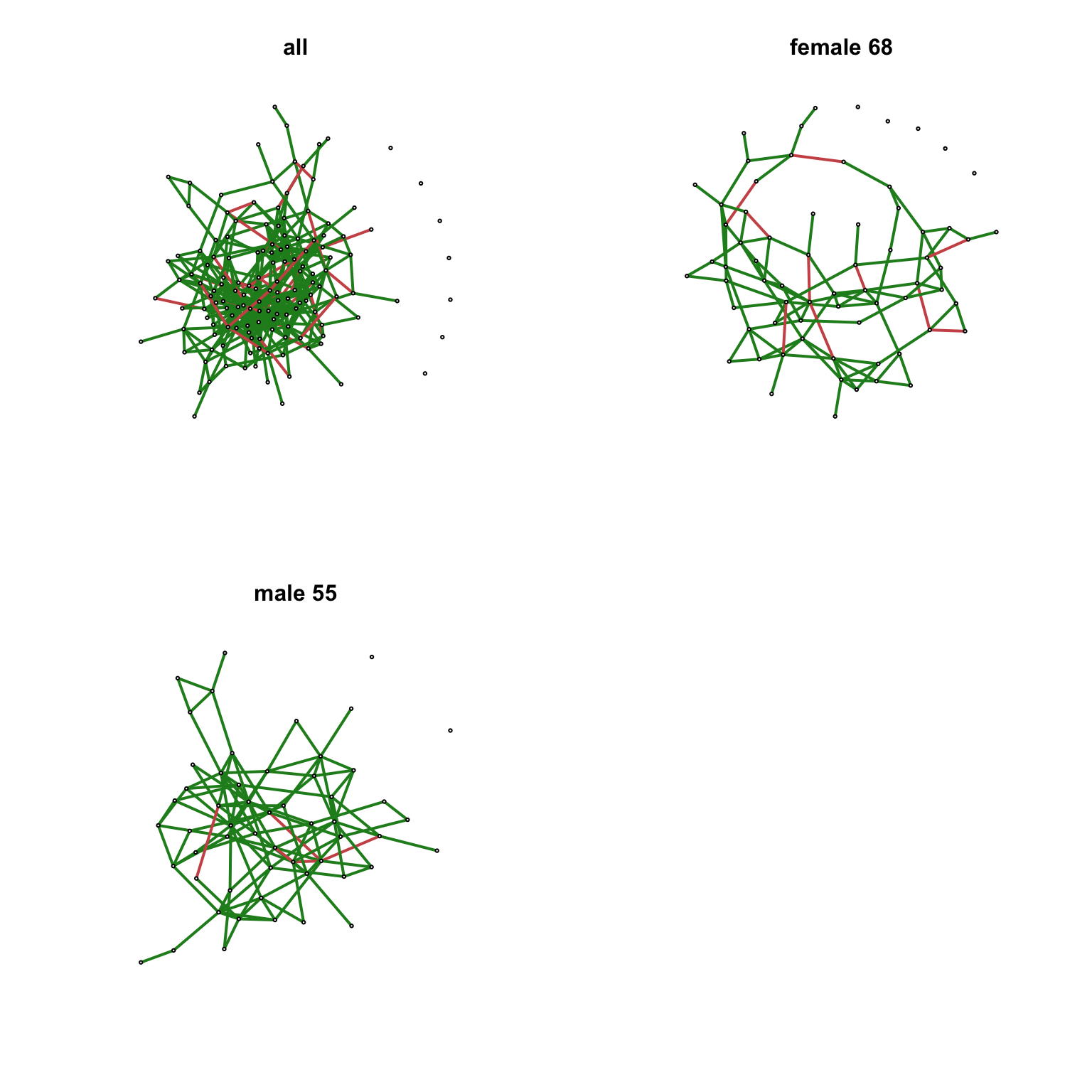

7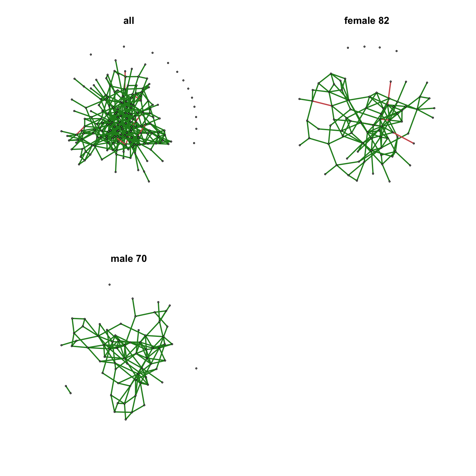

8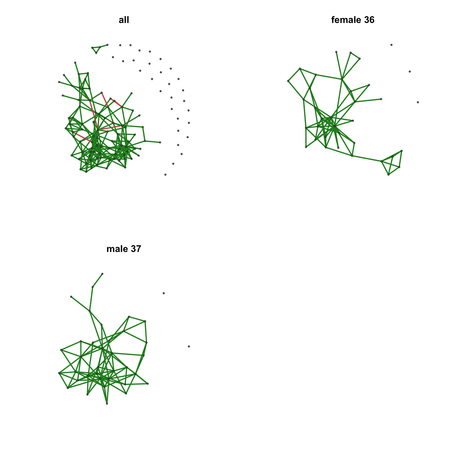

9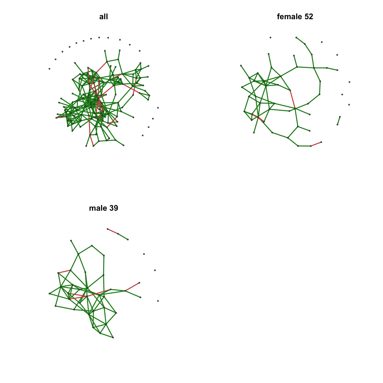

10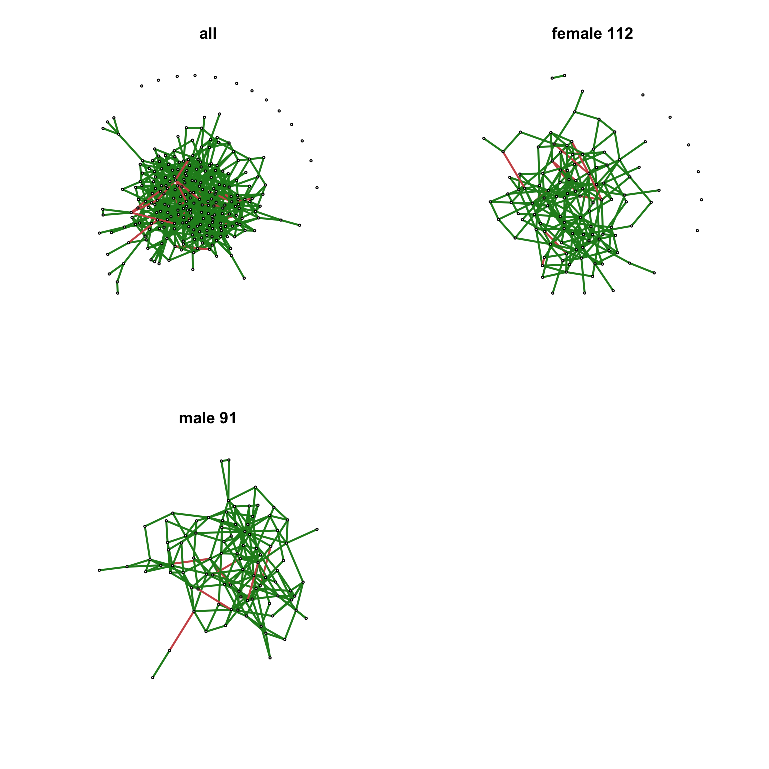

11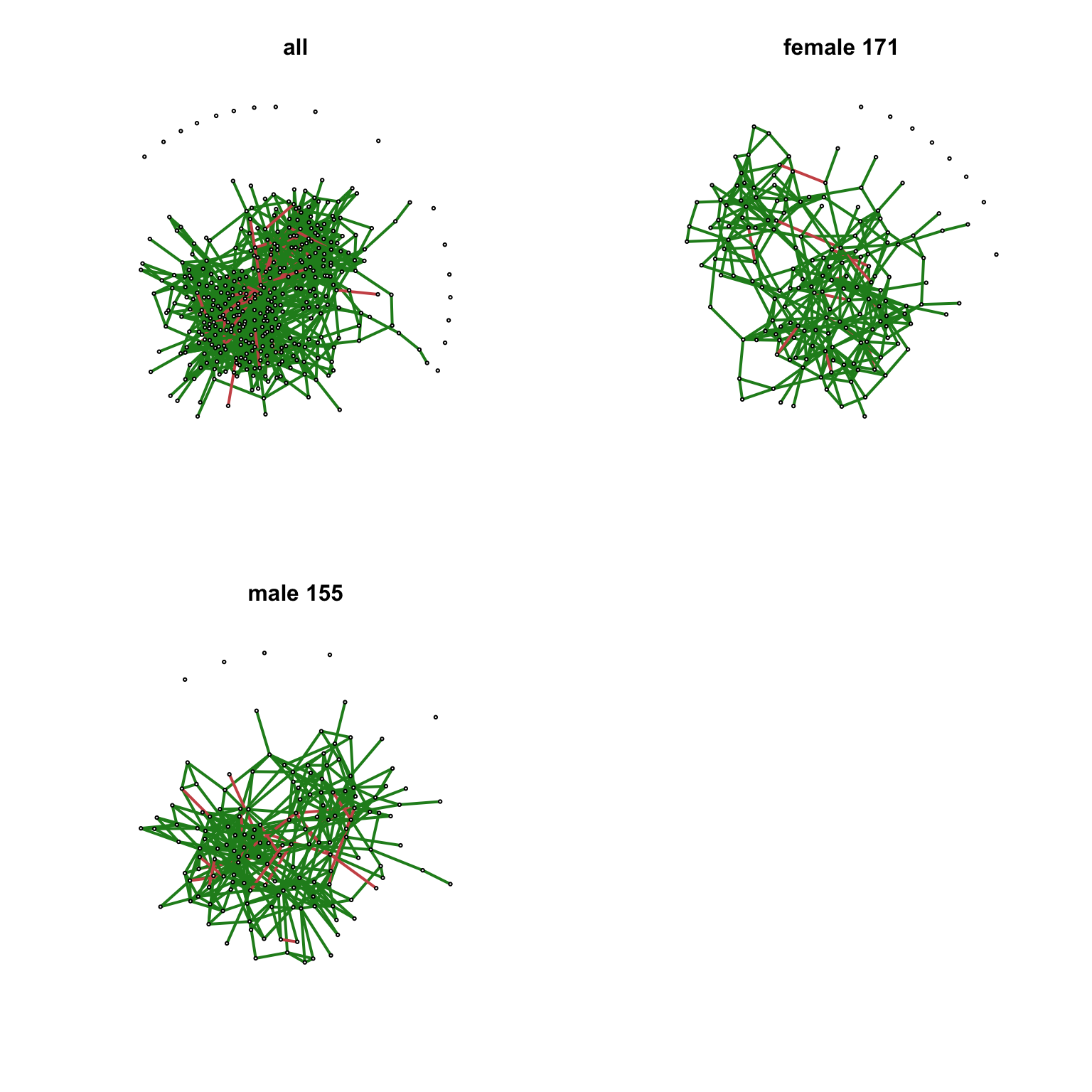

12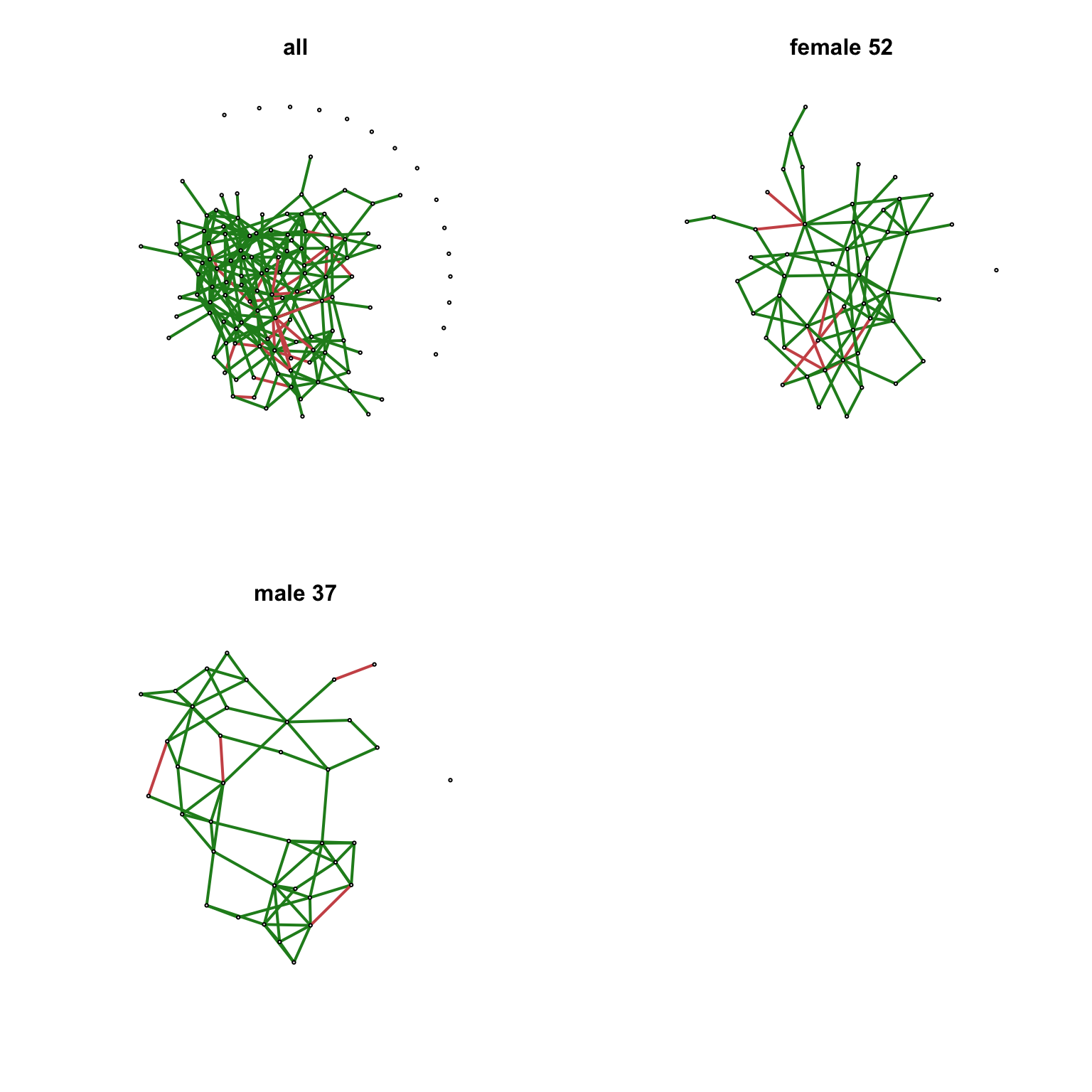

13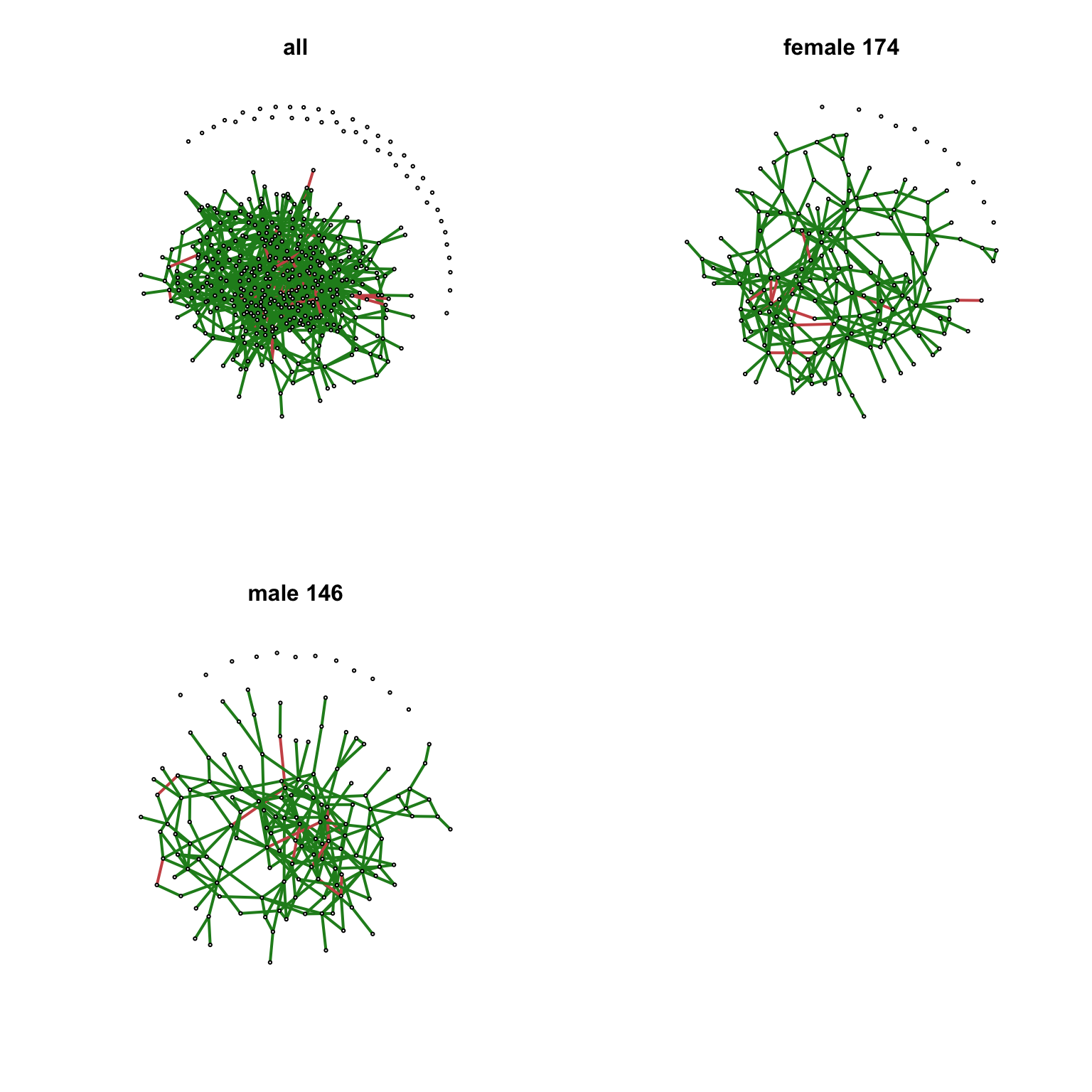

14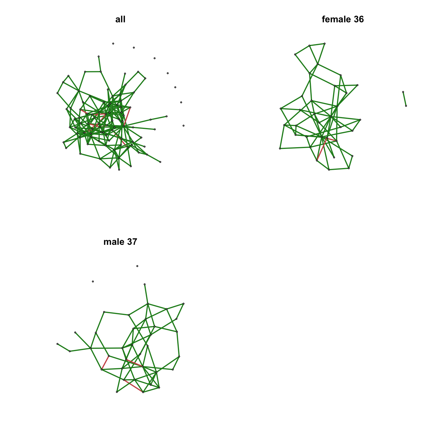

15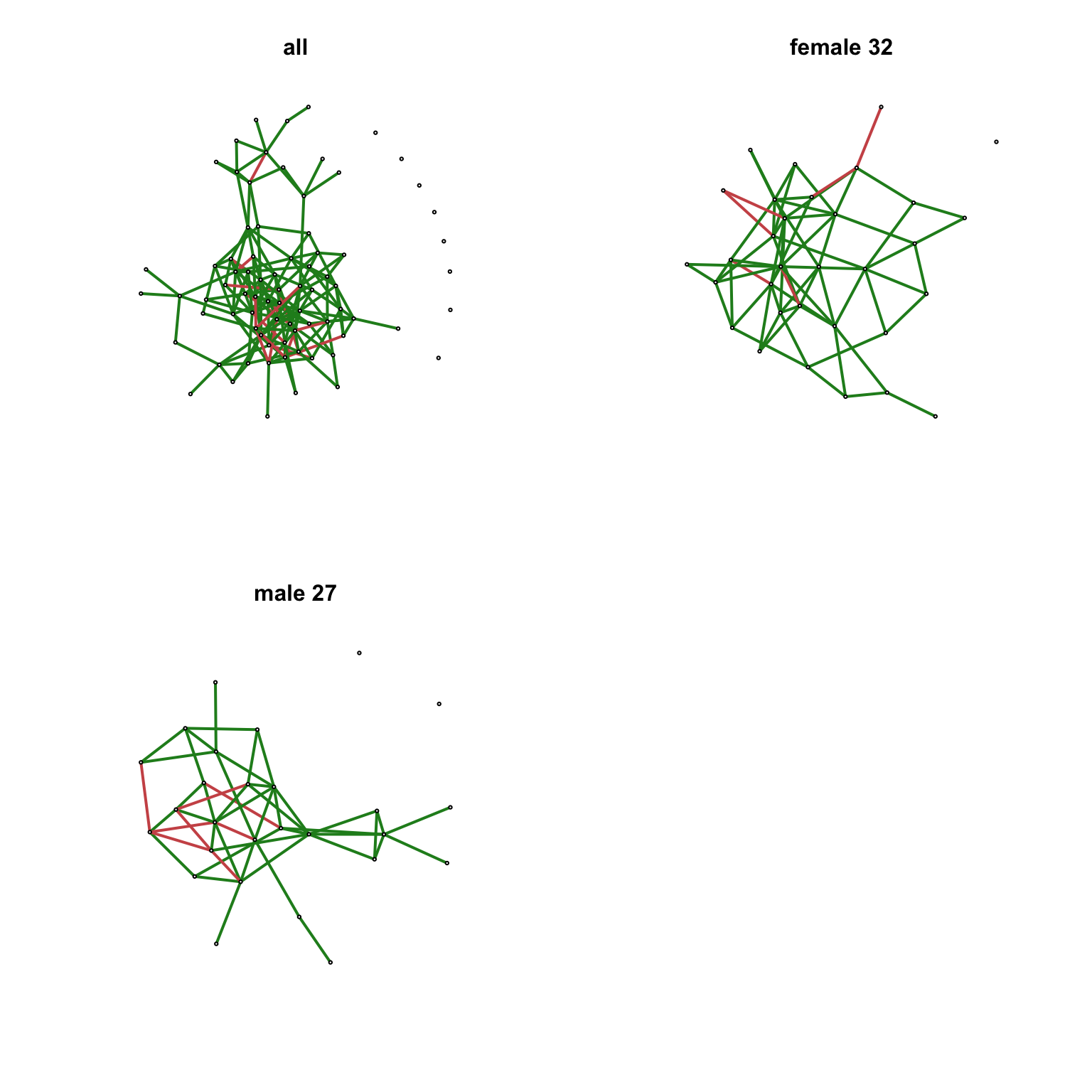

16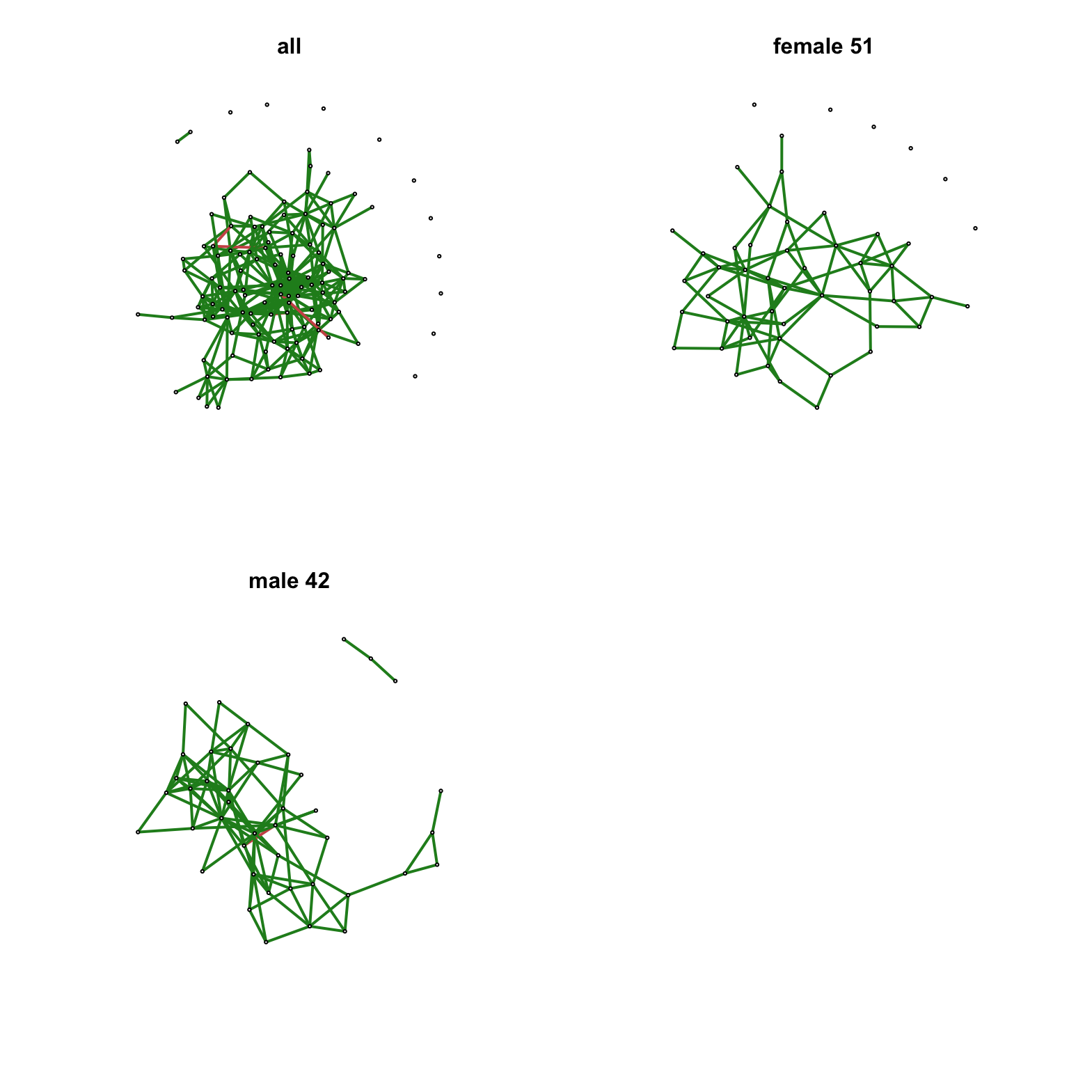

17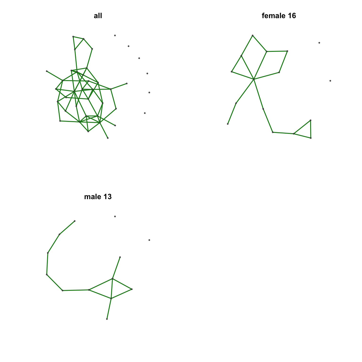

18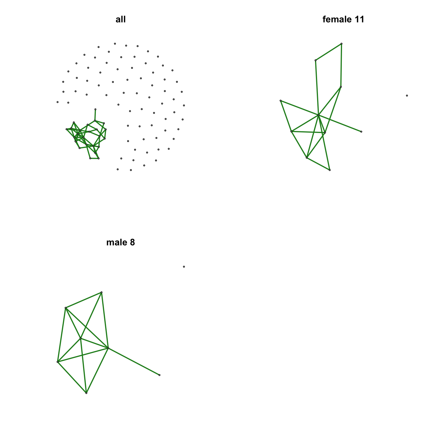

19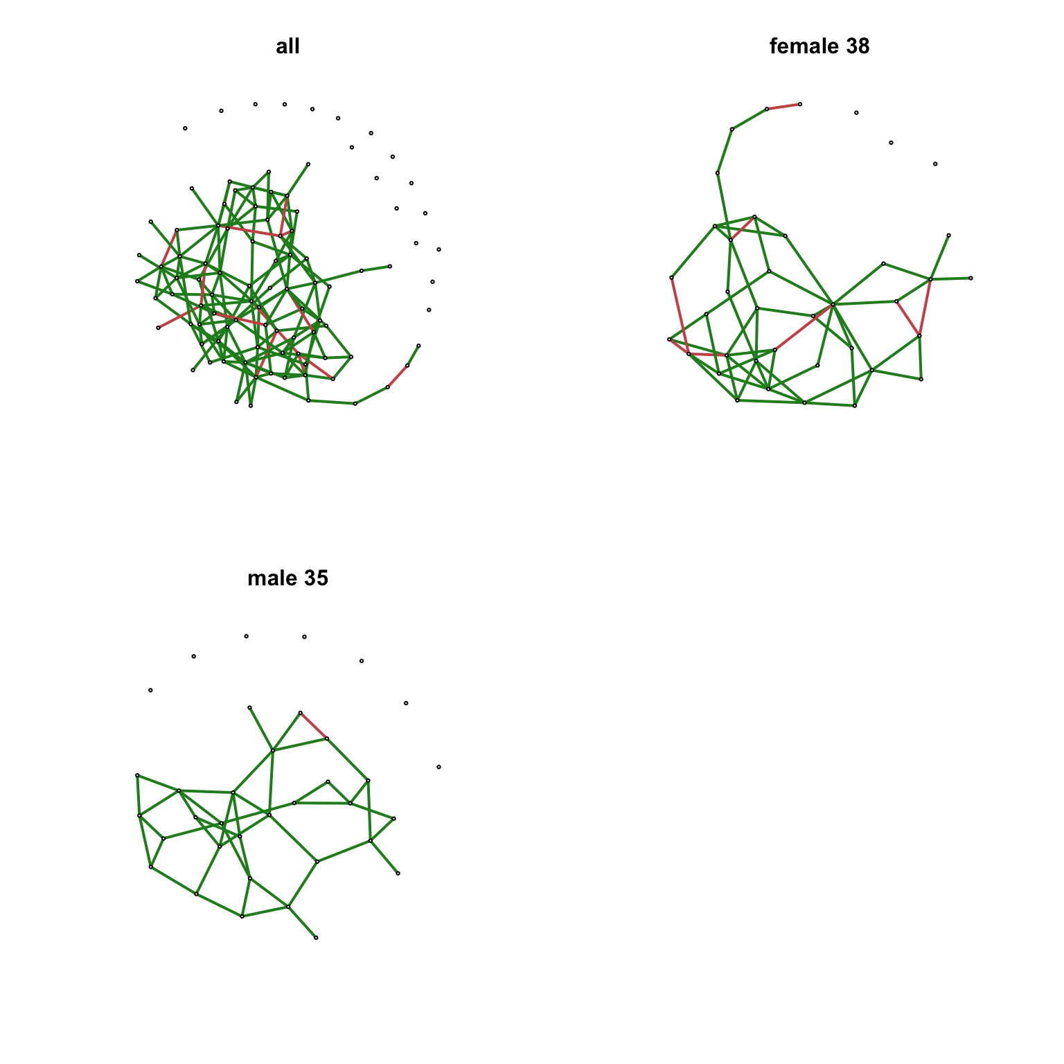

20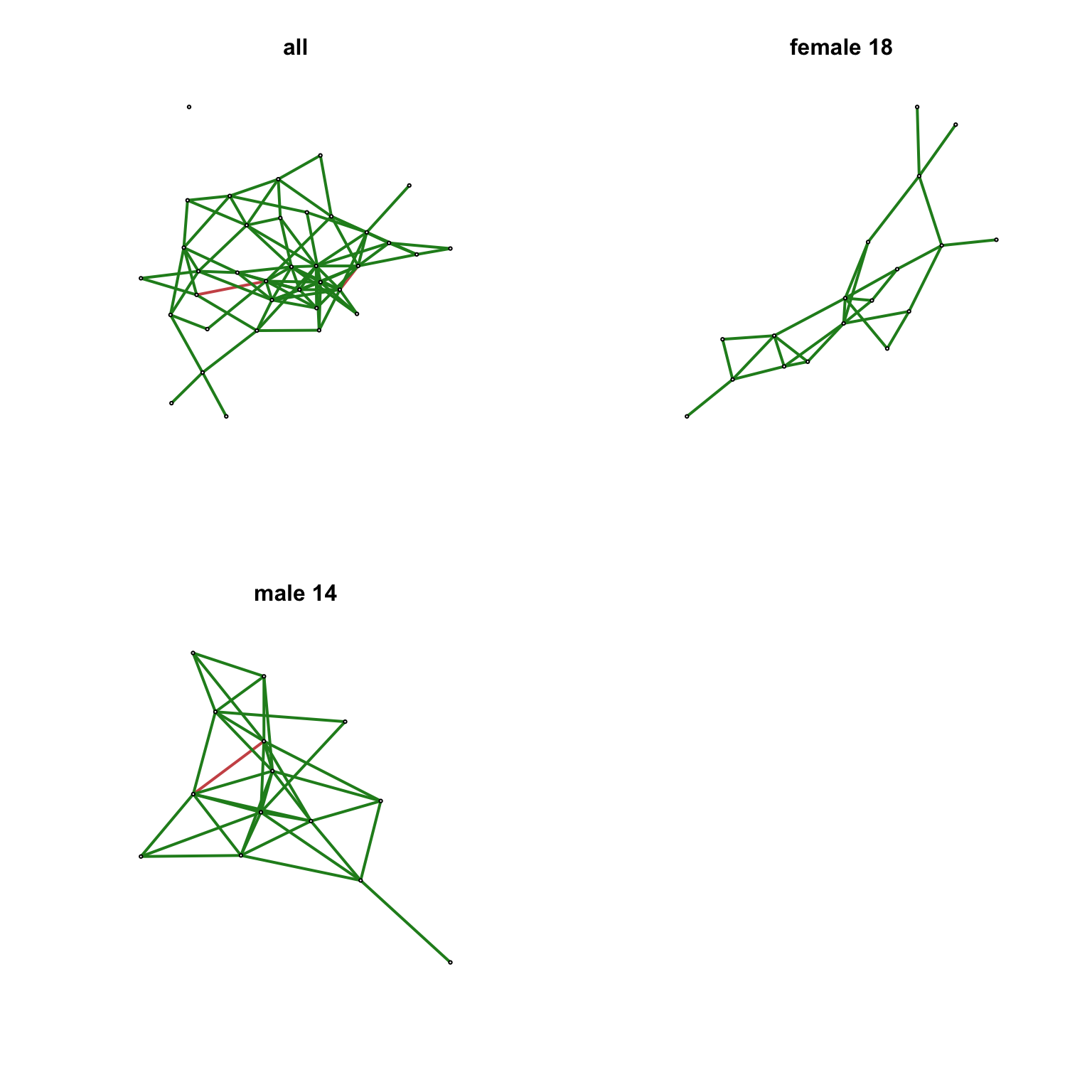

21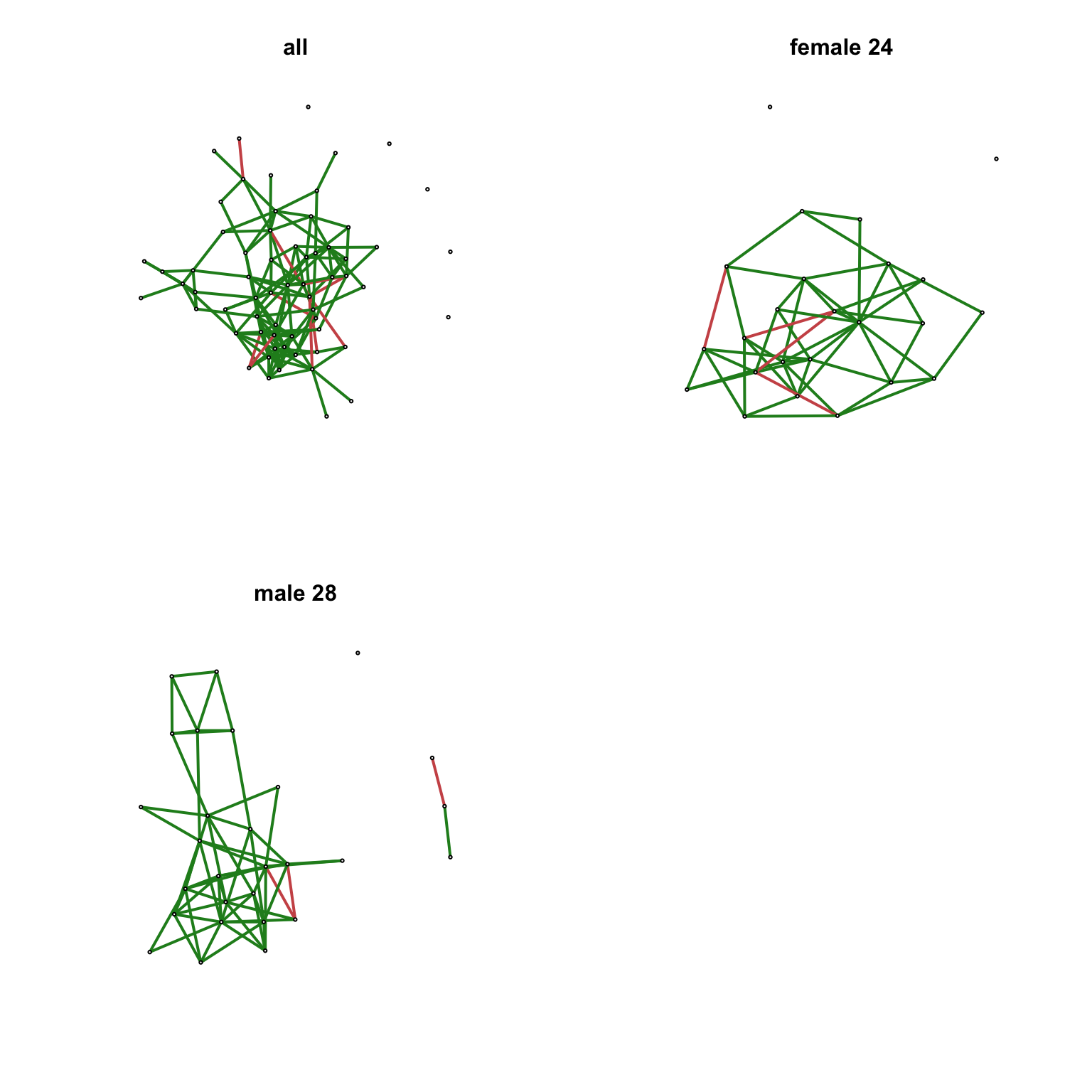

22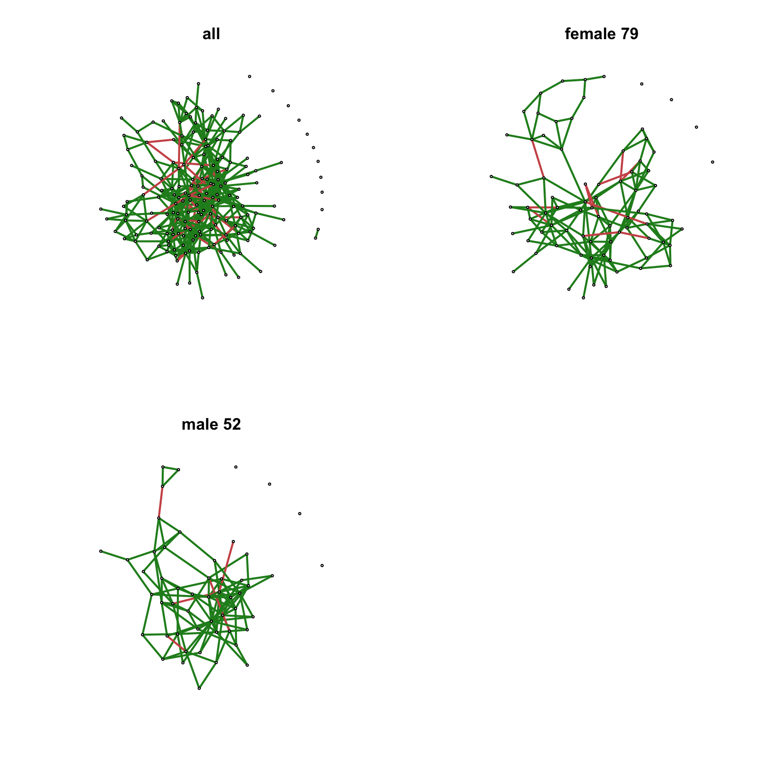

23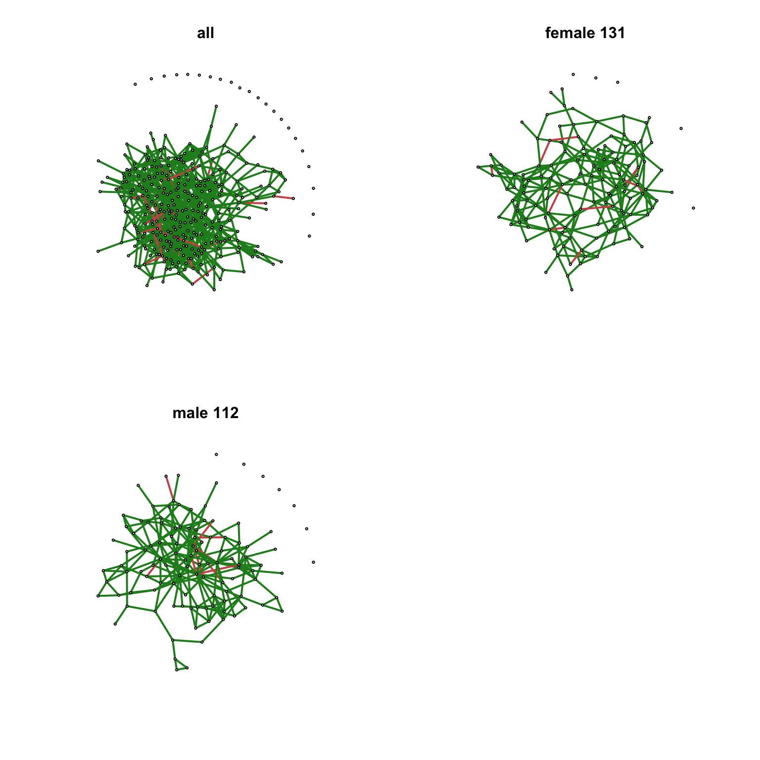

24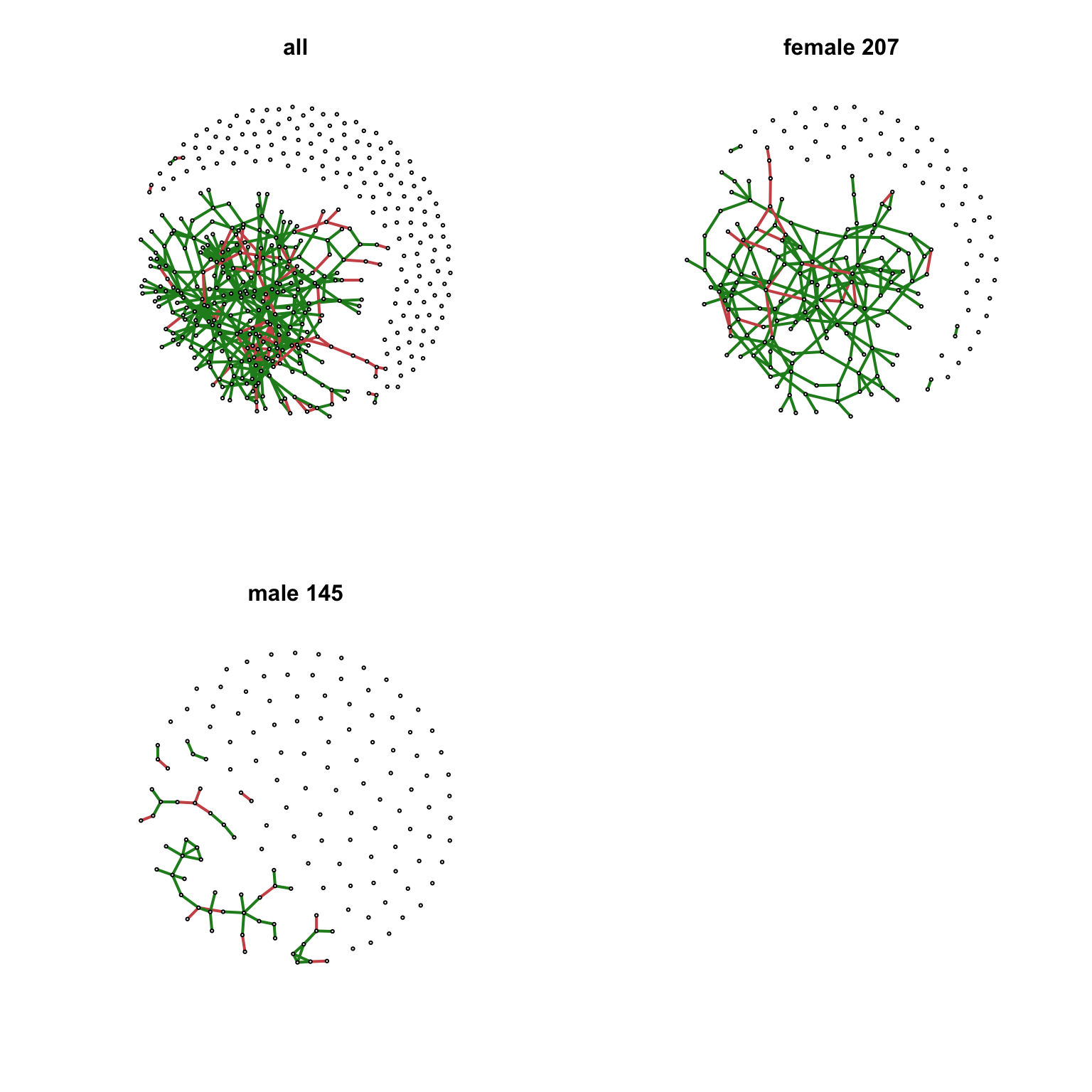

25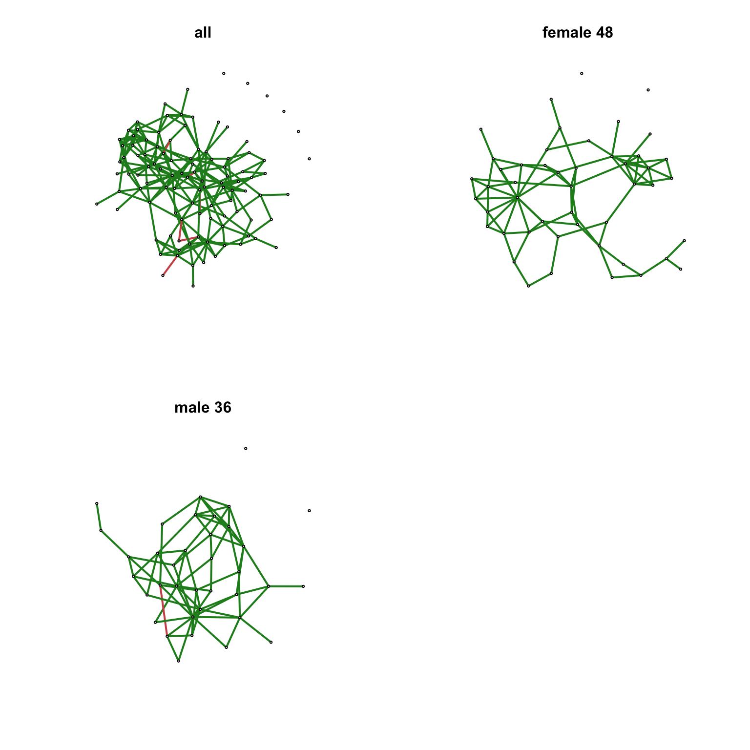

26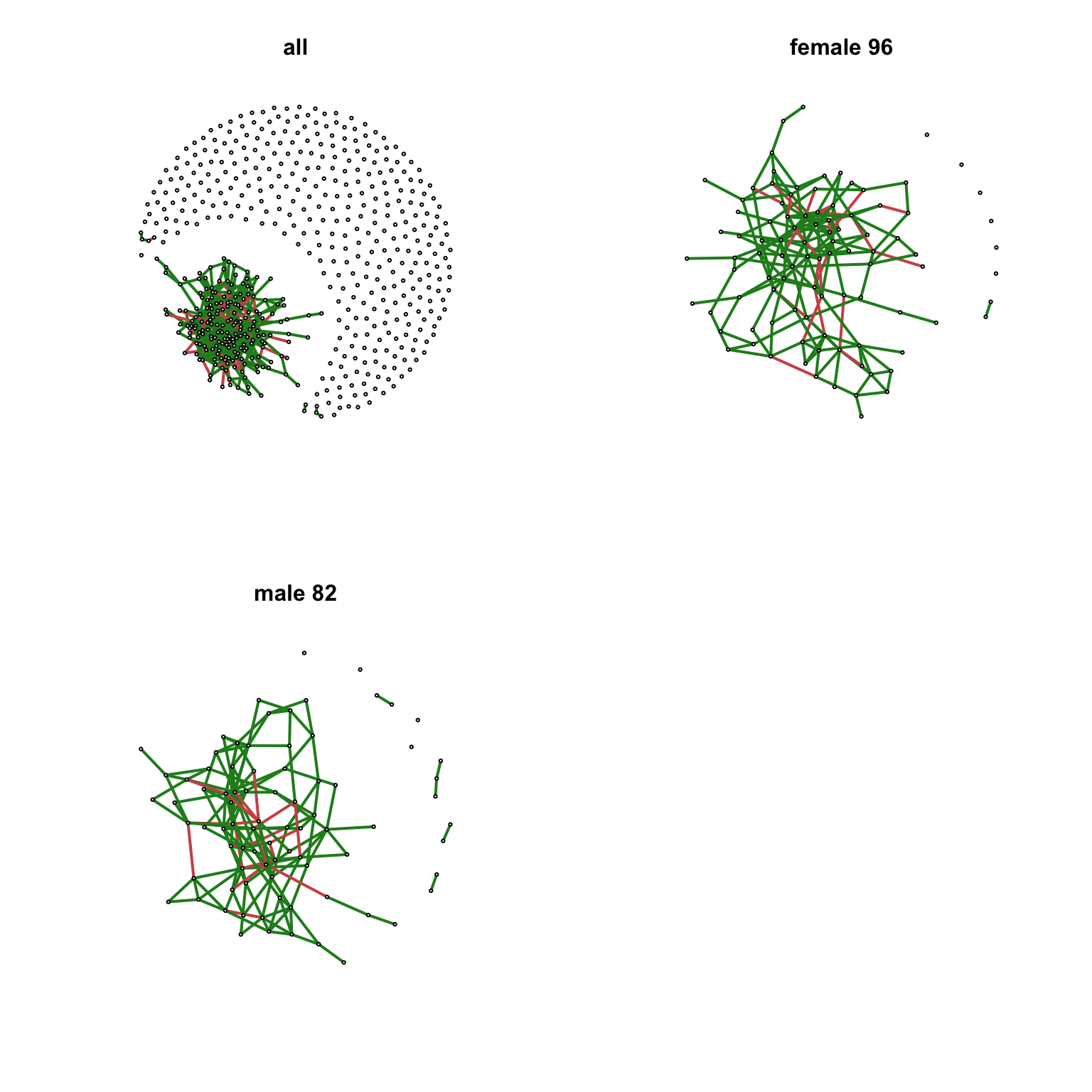

27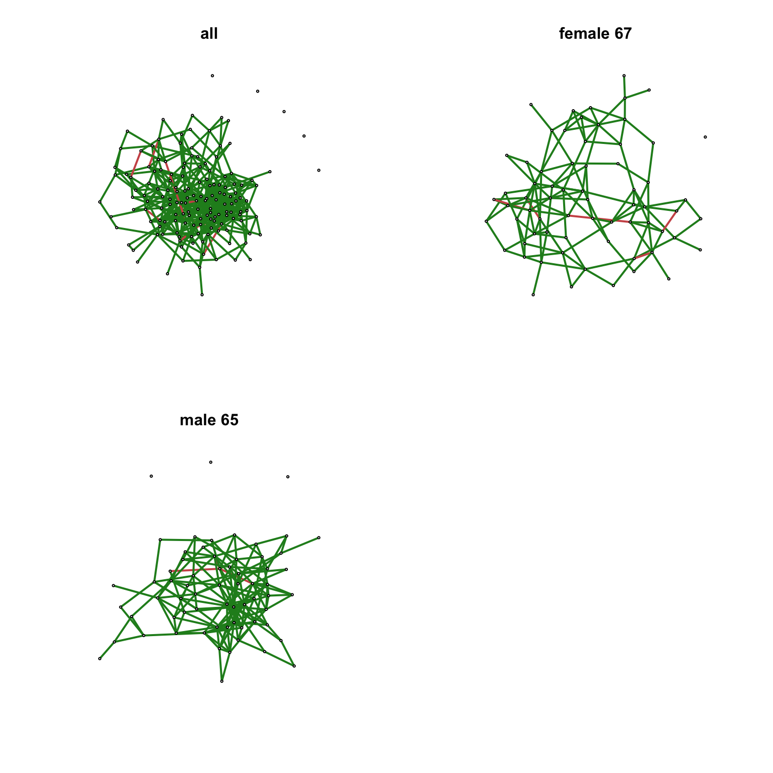

28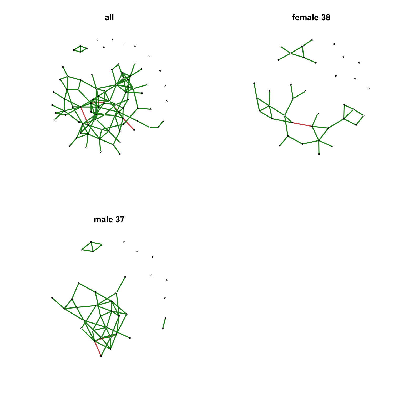

29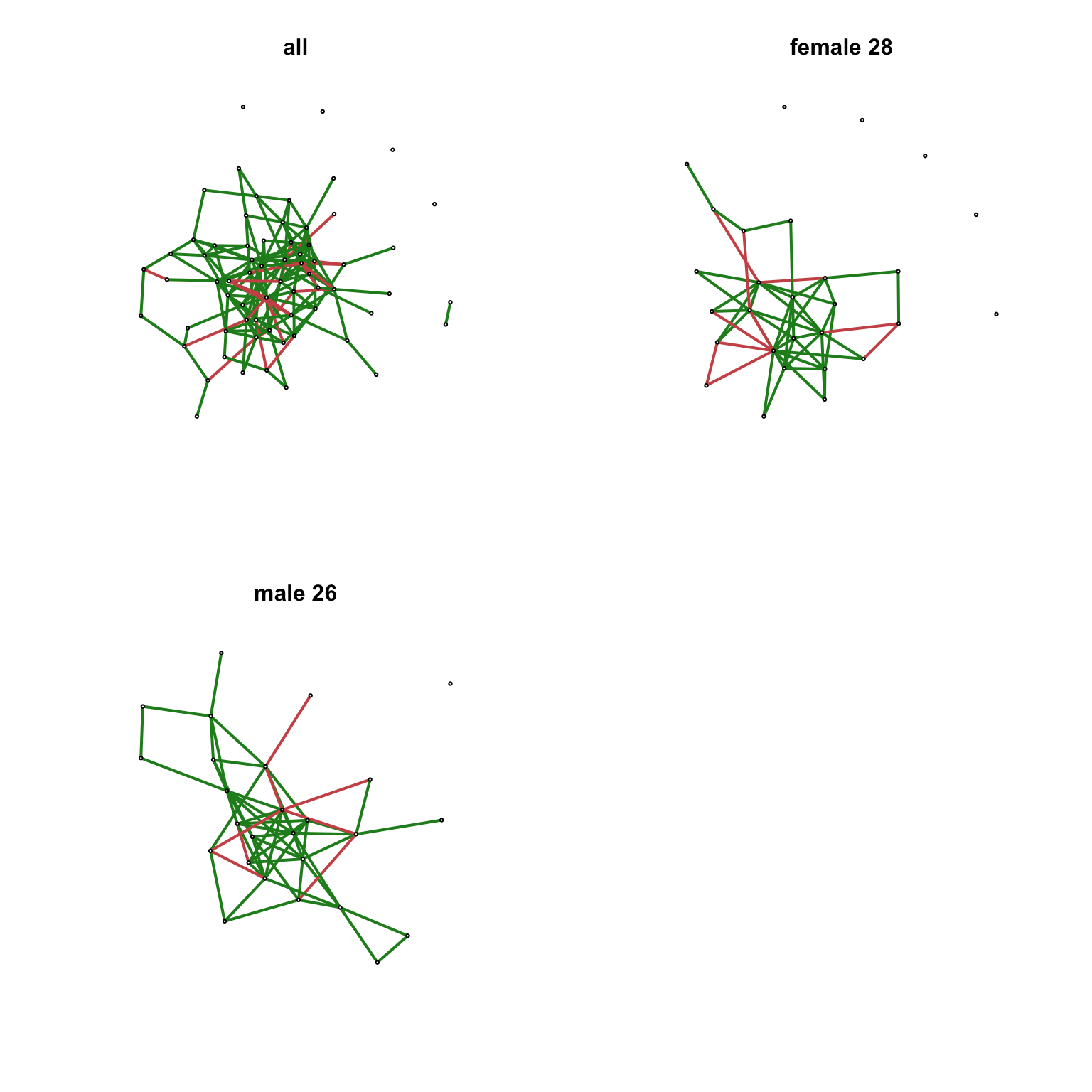

30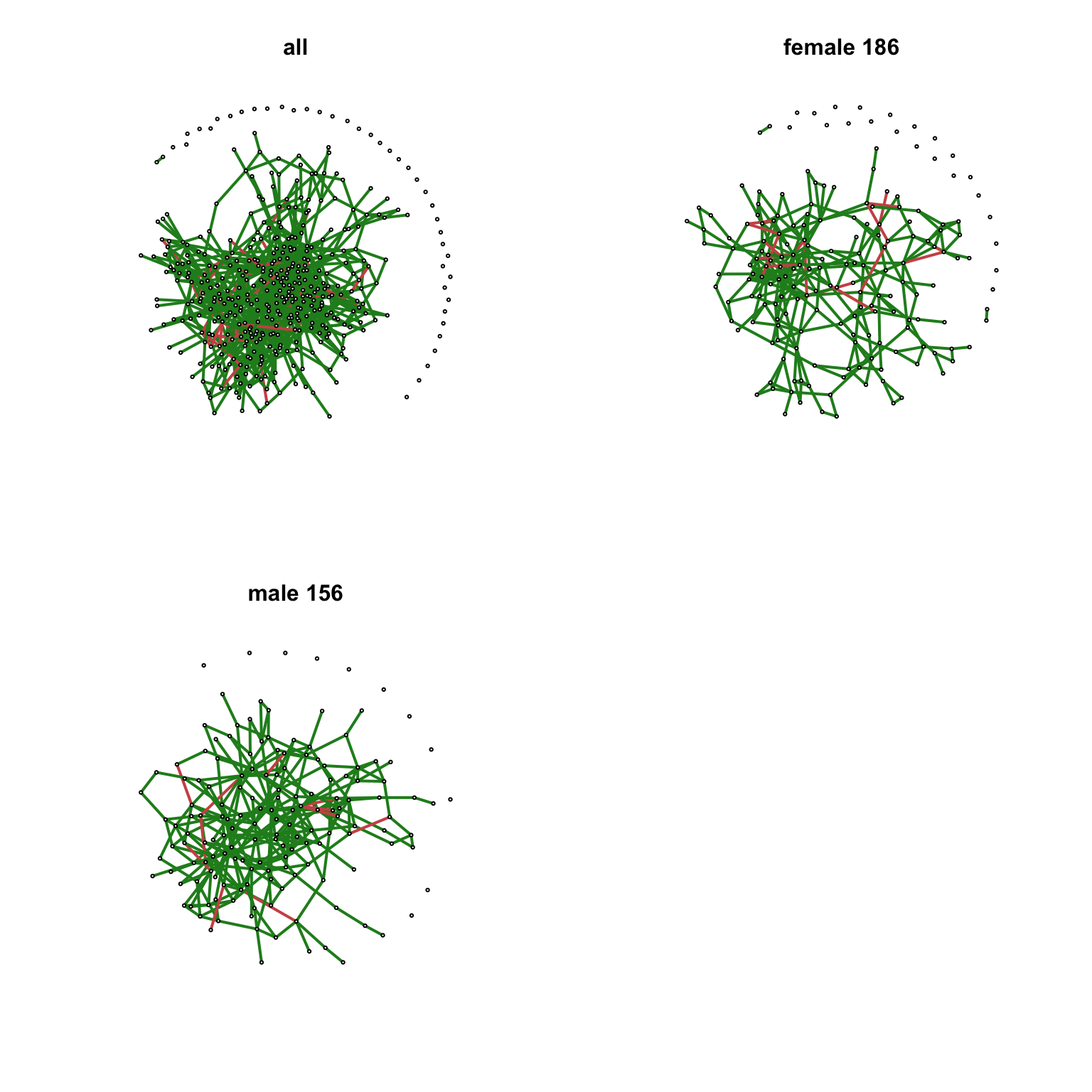

31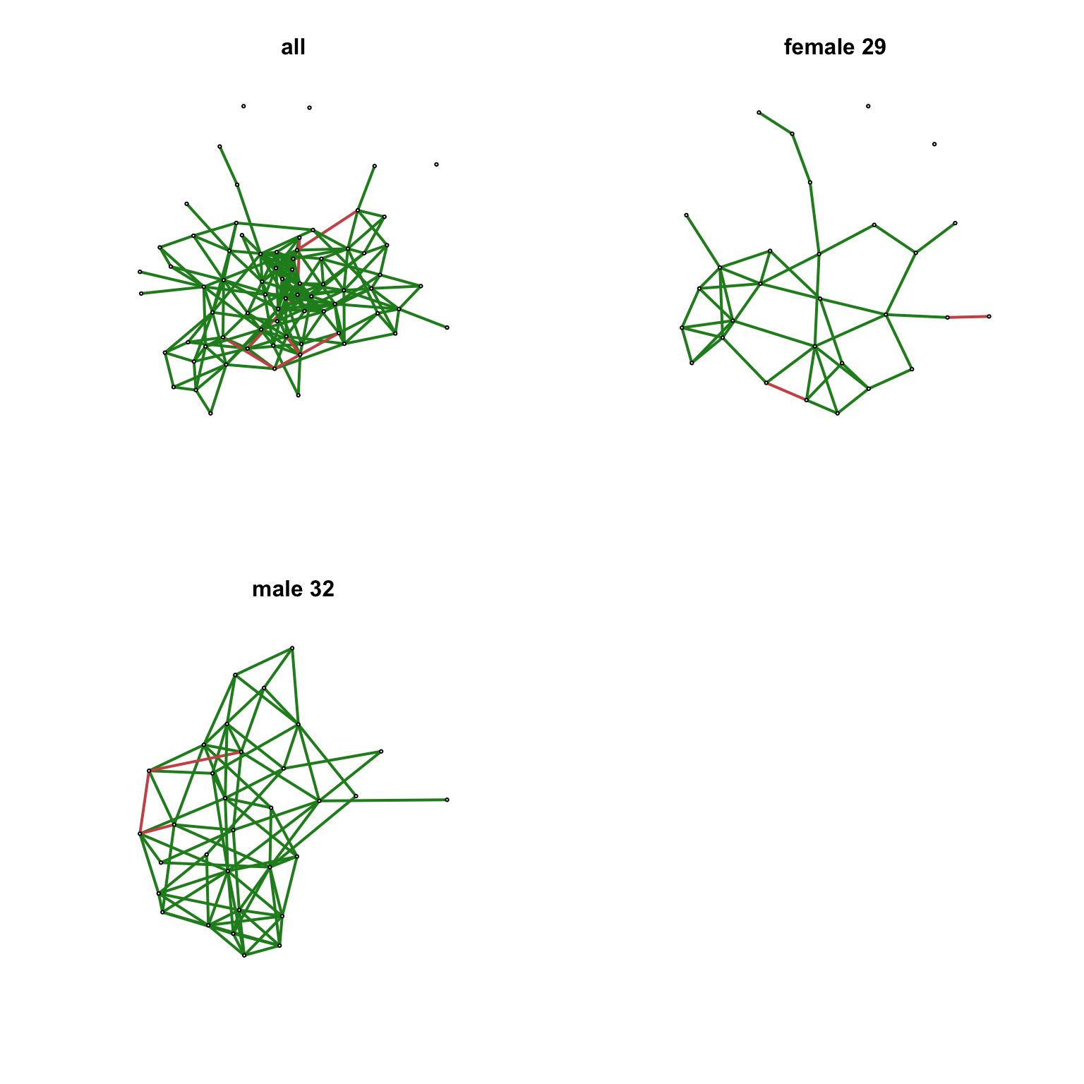

32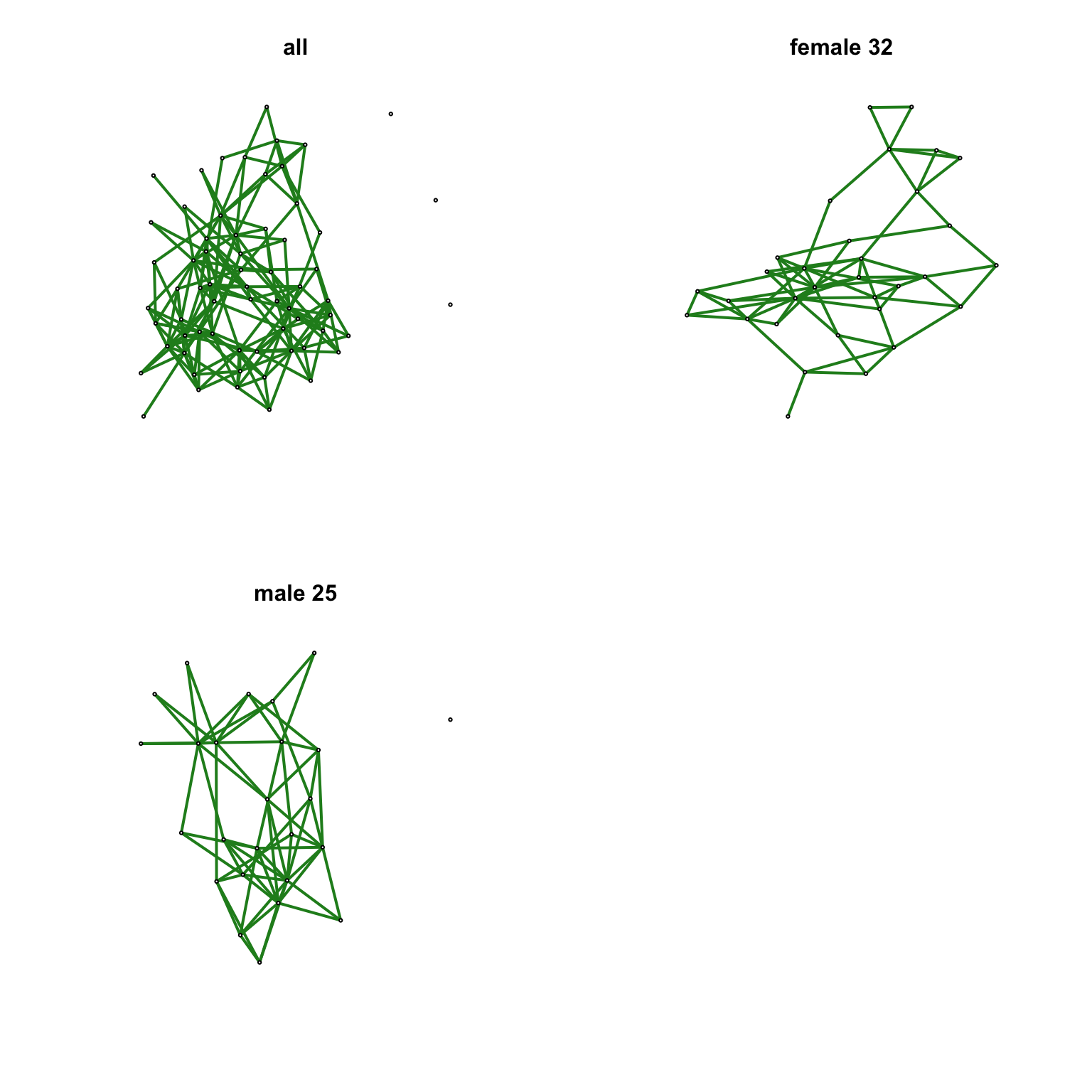

Cross Gender Negative Ties

00	01	10	11
159	87	80	204

00	01	10	11
3286	1047	1141	3509

Check

Linear Model

Call:
lm(formula = as.formula(paste("-strat.meas ~", paste(names(df)[10:13], 
    collapse = " + "))), data = df)

Residuals:
    Min      1Q  Median      3Q     Max 
-5.5975 -2.2036 -0.1374  1.5414  7.7995 

Coefficients:
             Estimate Std. Error t value Pr(>|t|)
(Intercept)  1.141191   1.146181   0.996    0.330
age10        0.024460   0.096560   0.253    0.802
age20        0.004219   0.035633   0.118    0.907
age50        0.083091   0.104862   0.792    0.436
age70       -0.158469   0.226088  -0.701    0.490

Residual standard error: 3.245 on 23 degrees of freedom
Multiple R-squared:  0.1808,    Adjusted R-squared:  0.03829 
F-statistic: 1.269 on 4 and 23 DF,  p-value: 0.3109

Let’s look at unbalanced triangles, and see where the genders lie.