Vertex Statistics
Linear Models
Let’s try to perform some linear models.
Call:
lm(formula = dni ~ dpi + bp + cp, data = bdf)

Residuals:
    Min      1Q  Median      3Q     Max
-0.4424 -0.1218 -0.0947 -0.0865  8.8919

Coefficients:
              Estimate Std. Error t value Pr(>|t|)
(Intercept)  8.662e-02  8.120e-03  10.667  < 2e-16 ***
dpi          7.216e-03  2.718e-03   2.655  0.00795 **
bp           2.169e-05  7.111e-06   3.050  0.00230 **
cp          -1.156e+01  1.514e+01  -0.764  0.44514
---
Signif. codes:  0 '***' 0.001 '**' 0.01 '*' 0.05 '.' 0.1 ' ' 1

Residual standard error: 0.447 on 5855 degrees of freedom
Multiple R-squared:  0.007258,  Adjusted R-squared:  0.006749
F-statistic: 14.27 on 3 and 5855 DF,  p-value: 2.918e-09
Call:
lm(formula = dni ~ dpi, data = bdf)

Residuals:
    Min      1Q  Median      3Q     Max
-0.4296 -0.1301 -0.0955 -0.0840  8.8930

Coefficients:
            Estimate Std. Error t value Pr(>|t|)
(Intercept) 0.083995   0.007941  10.578  < 2e-16 ***
dpi         0.011521   0.002087   5.521 3.52e-08 ***
---
Signif. codes:  0 '***' 0.001 '**' 0.01 '*' 0.05 '.' 0.1 ' ' 1

Residual standard error: 0.4474 on 5857 degrees of freedom
Multiple R-squared:  0.005177,  Adjusted R-squared:  0.005007
F-statistic: 30.48 on 1 and 5857 DF,  p-value: 3.519e-08
Call:
lm(formula = dni ~ bp, data = bdf)

Residuals:
    Min      1Q  Median      3Q     Max
-0.5191 -0.1108 -0.0971 -0.0971  8.8920

Coefficients:
             Estimate Std. Error t value Pr(>|t|)
(Intercept) 9.709e-02  6.468e-03  15.012  < 2e-16 ***
bp          3.325e-05  5.566e-06   5.975 2.44e-09 ***
---
Signif. codes:  0 '***' 0.001 '**' 0.01 '*' 0.05 '.' 0.1 ' ' 1

Residual standard error: 0.4472 on 5857 degrees of freedom
Multiple R-squared:  0.006058,  Adjusted R-squared:  0.005888
F-statistic:  35.7 on 1 and 5857 DF,  p-value: 2.441e-09
Call:
lm(formula = dni ~ cp, data = bdf)

Residuals:
    Min      1Q  Median      3Q     Max
-0.1150 -0.1150 -0.1146 -0.1129  8.8850

Coefficients:
             Estimate Std. Error t value Pr(>|t|)
(Intercept)  0.114993   0.006529  17.614   <2e-16 ***
cp          -6.508950  14.175694  -0.459    0.646
---
Signif. codes:  0 '***' 0.001 '**' 0.01 '*' 0.05 '.' 0.1 ' ' 1

Residual standard error: 0.4485 on 5857 degrees of freedom
Multiple R-squared:  3.6e-05,   Adjusted R-squared:  -0.0001347
F-statistic: 0.2108 on 1 and 5857 DF,  p-value: 0.6461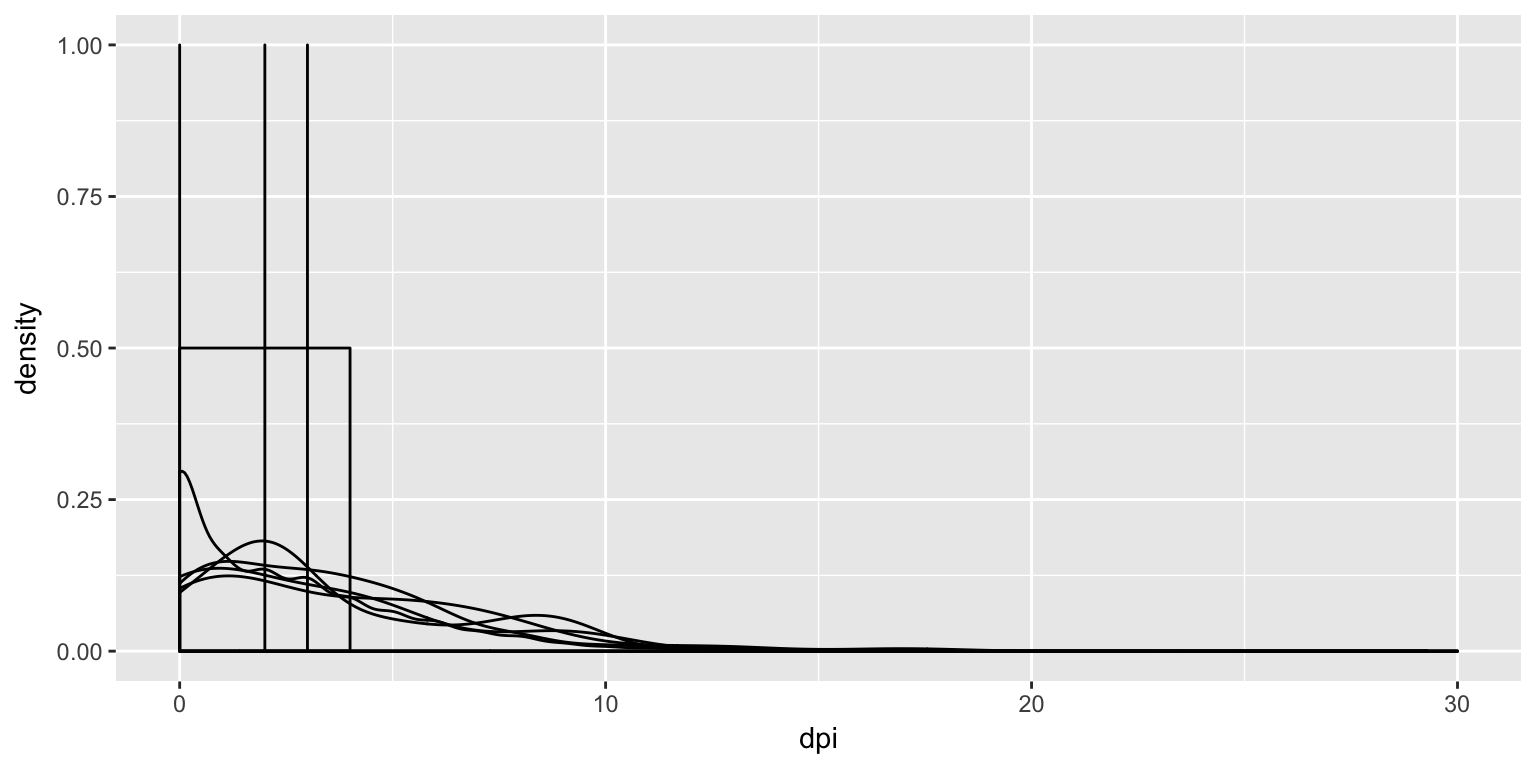
So, an untrained individual would rejoice at such results. The problem is that we’re dealing with such heavy tailed distributions that conclusions from linear models are just not going to be useful.
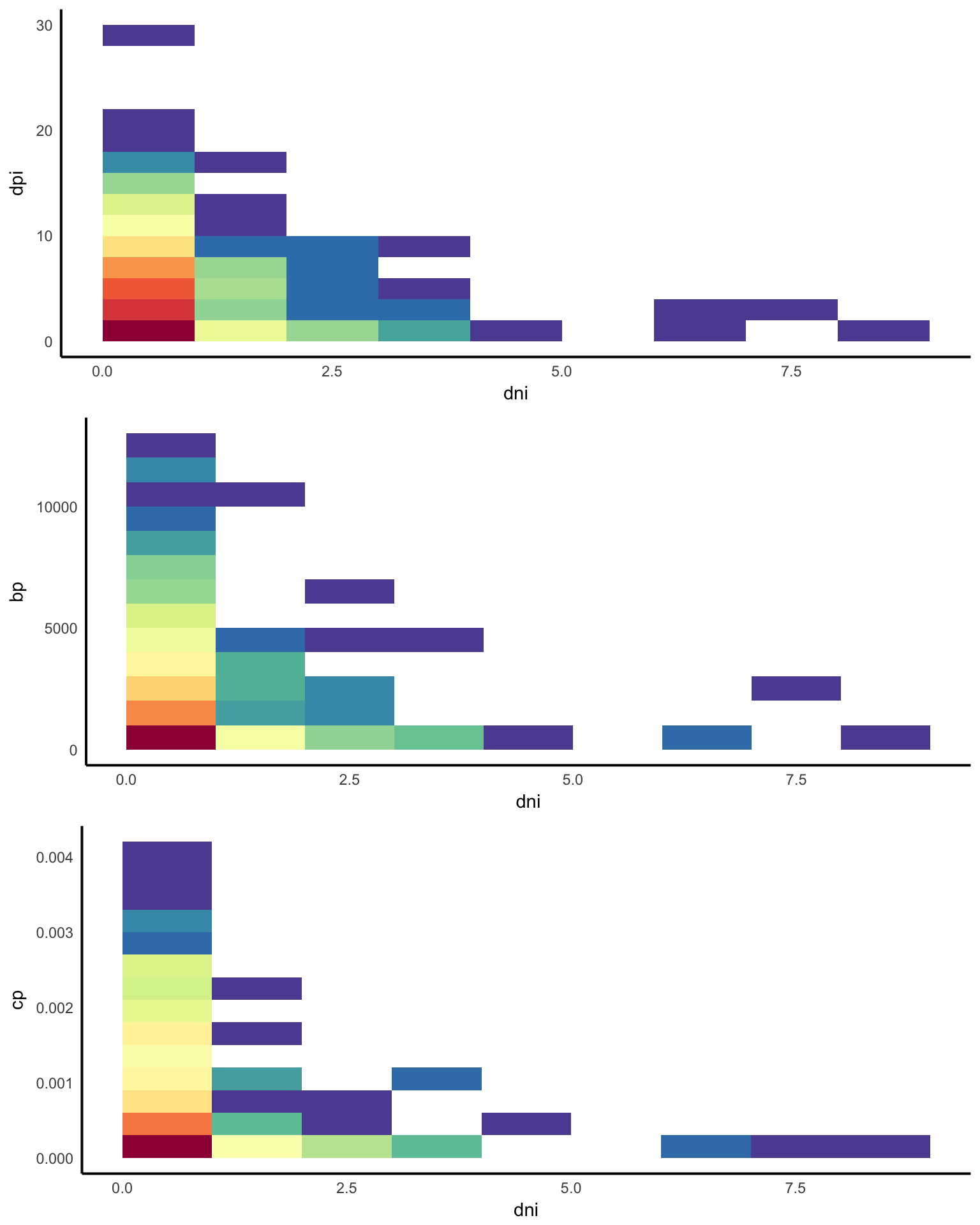
Heatmaps
So this was a fun exercise in making heatmaps, trying to an inverse relationship between the number of negative in-ties of a person, and some other covariate. The problem is that when the data drops considerably but has a pretty long tale, then it’s going to look sort of like there’s an inverse relationship, when in fact it’s more likely just pure chance.
Shortest Paths
Intuitively, we should see something like the shortest path in the positive subgraph is longer if the tie is a negative tie.
Let’s do \(t\)-tests:
| i | estimate | p.value | stars | estimate1 | estimate2 | statistic |
|---|---|---|---|---|---|---|
| 1 | -0.434 | 0.248 | 3.000 | 3.434 | -1.321 | |
| 2 | 2.351 | 0.045 | * | 5.636 | 3.286 | 2.280 |
| 4 | 6.736 | 0.285 | 14.333 | 7.597 | 1.435 | |
| 5 | 3.774 | 0.034 | * | 9.083 | 5.309 | 2.415 |
| 6 | -0.390 | 0.290 | 3.471 | 3.860 | -1.072 | |
| 7 | 0.455 | 0.605 | 4.455 | 4.000 | 0.533 | |
| 8 | 1.043 | 0.185 | 4.500 | 3.457 | 1.511 | |
| 9 | -0.194 | 0.722 | 4.250 | 4.444 | -0.359 | |
| 10 | 3.019 | 0.002 | ** | 6.750 | 3.731 | 3.387 |
| 11 | 0.256 | 0.458 | 4.069 | 3.813 | 0.746 | |
| 12 | 1.332 | 0.085 | . | 5.625 | 4.293 | 1.794 |
| 13 | 0.931 | 0.047 | * | 4.949 | 4.018 | 2.050 |
| 14 | -1.151 | 0.001 | *** | 2.250 | 3.401 | -4.208 |
| 15 | -0.665 | 0.110 | 3.000 | 3.665 | -1.658 | |
| 16 | 2.173 | 0.281 | 5.500 | 3.327 | 1.309 | |
| 19 | 0.236 | 0.794 | 4.467 | 4.230 | 0.266 | |
| 20 | 0.022 | 0.986 | 3.000 | 2.978 | 0.022 | |
| 21 | 1.287 | 0.109 | 4.700 | 3.413 | 1.766 | |
| 22 | 0.284 | 0.534 | 4.053 | 3.768 | 0.627 | |
| 23 | 0.539 | 0.213 | 4.333 | 3.794 | 1.269 | |
| 24 | 3.304 | 0.000 | *** | 11.324 | 8.019 | 4.971 |
| 25 | 2.432 | 0.165 | 5.857 | 3.425 | 1.580 | |
| 26 | 1.016 | 0.044 | * | 5.312 | 4.296 | 2.037 |
| 27 | -0.247 | 0.603 | 3.167 | 3.414 | -0.534 | |
| 28 | 1.769 | 0.566 | 7.000 | 5.231 | 0.640 | |
| 29 | 0.094 | 0.840 | 3.826 | 3.732 | 0.203 | |
| 30 | 1.257 | 0.030 | * | 5.750 | 4.493 | 2.222 |
| 31 | -0.544 | 0.084 | . | 2.625 | 3.169 | -1.945 |
Add in the results for stratified measure.
Common Enemies?
TODO