Change Blindness
Humans are surprisingly bad at noticing things if their attention is diverted or arrested. Examples I’ve come across include this video of basketball pass counts and Derren Brown’s people swap. Known as change blindness, this is a well studied phenomenon in Psychology literature. The thesis we are interested in today is the following:
A person’s propensity towards alignment change blindness is correlated with their preference towards images of alignment versus misalignments
In other words, we expect that a person’s ability to detect changes involving misalignments (measured here in response time) should correlate with their preference for aligned images over misaligned ones.
This is a fairly involved study, for the following reasons:
In order to determine a peron’s ability to detect changes involving misalignments, we need to compare it to some base change detection ability. The reasoning here is that perhaps the person is just good at detecting all forms of changes.
As we’ll see later on, different images have different baseline difficulty levels when it comes to change blindness, so the response variables must take that into account.
Preprocessing
In this section, we’ll load and clean the data for processing.
Loading in the data:
cb.all <- c()
pre.all <- c()

for (i in 1:3) {
  cb <- read.csv(paste0("data/cb", i, ".csv"))
  pre <- read.csv(paste0("data/pre", i, ".csv"))

  # adding round
  cb$round <- i
  pre$round <- i

  cb.all <- rbind(cb.all, cb)
  pre.all <- rbind(pre.all, pre)
}
Now we need to do some cleaning:
# cleaning change blindness
#  - remove missing data
#  - fixing image numbers for round 2:
#    (changed them to 10 + imageNum)
cb.all <- cb.all %>%
  filter(!is.na(Acc) & !is.na(clickX)) %>%
  mutate_each(funs(as.integer), clickX, clickY, imageNum) %>%
  mutate(
    imageNum = ifelse(round == 2, 10+imageNum, imageNum),
    image = paste(imageNum, misalign., sep="."),
    misalign = ifelse(misalign. == 1, "misalign", "other")
    ) %>%
  select(-workerID)

# cleaning preference
pre.all <- pre.all %>%
  mutate(
    c1 = grepl("c1", imgNum),
    c0 = grepl("c0", imgNum),
    f = grepl("f", imgNum),
    x = grepl("x", imgNum),
    o = grepl("^o", imgNum),
    ori = grepl("_o", imgNum),
    img.num = as.integer(sub("^[^c]([0-9]+).*$", "\\1", imgNum))
    )
pre.all <- pre.all %>%
  mutate(type = apply(.[,8:13], 1, function(x) {
    names(pre.all)[8:13][which.max(x)]
  })) %>%
  select(-c1, -c0, -f, -x, -o, -ori, -workerID)
It will be helpful to classify subjects into groups with the same treatments.
cb <- cb.all %>%
  filter(Acc == 1)
sub1 <- cb %>%
  filter(image=="1.0") %>%
  select(subNum) %>%
  unique %>%
  arrange(subNum) %>%
  .$subNum
sub2 <- cb %>%
  filter(image=="1.1") %>%
  select(subNum) %>%
  unique %>%
  arrange(subNum) %>%
  .$subNum
sub3 <- cb %>%
  filter(image=="11.0") %>%
  select(subNum) %>%
  unique %>%
  arrange(subNum) %>%
  .$subNum
sub4 <- cb %>%
  filter(image=="11.1") %>%
  select(subNum) %>%
  unique %>%
  arrange(subNum) %>%
  .$subNum
Preanalysis
CB study
Let’s look things by images first. The table below shows the median response times for the misaligned version and the other version per image, as well as the difference between the two medians.1 Note that we have designated image numbers 11-20 to be from round 2 to differentiate those from the other two rounds. Clearly, we see that there is an image effect, in that the different images have different inherent difficulty levels.
| imageNum | misalign | other | diff |
|---|---|---|---|
| 1 | 17.2940 | 6.8210 | 10.4730 |
| 2 | 5.6100 | 12.5760 | -6.9660 |
| 3 | 5.9860 | 4.8915 | 1.0945 |
| 4 | 15.4810 | 19.7260 | -4.2450 |
| 5 | 14.0430 | 21.8760 | -7.8330 |
| 6 | 10.1050 | 13.1180 | -3.0130 |
| 7 | 6.5315 | 11.5880 | -5.0565 |
| 8 | 4.8180 | 5.1020 | -0.2840 |
| 9 | 4.0145 | 5.4745 | -1.4600 |
| 10 | 5.4495 | 4.5110 | 0.9385 |
| 11 | 14.6690 | 8.7350 | 5.9340 |
| 12 | 6.0140 | 8.5840 | -2.5700 |
| 13 | 6.3330 | 44.3745 | -38.0415 |
| 14 | 9.7300 | 16.7380 | -7.0080 |
| 15 | 14.8835 | 11.3570 | 3.5265 |
| 16 | 9.5690 | 5.0780 | 4.4910 |
| 17 | 8.7120 | 9.5360 | -0.8240 |
| 18 | 5.2740 | 3.3280 | 1.9460 |
| 19 | 5.5170 | 3.0540 | 2.4630 |
| 20 | 11.8660 | 3.0090 | 8.8570 |
A plot might be more informative. Unsurprisingly for a variable like response time, things are pretty variable, and there are plenty of outliers. Certain images like 4 and 5 display exaggerated variability. This might be what we want though, because we are after all trying to differentiate between people.2 The question as always is, how do we seperate the signal from the noise?
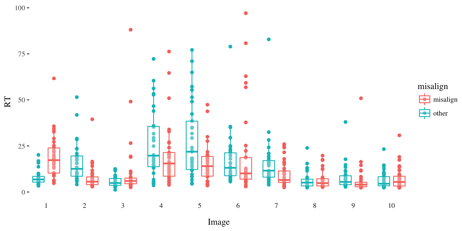
Distribution of Response Time per Image
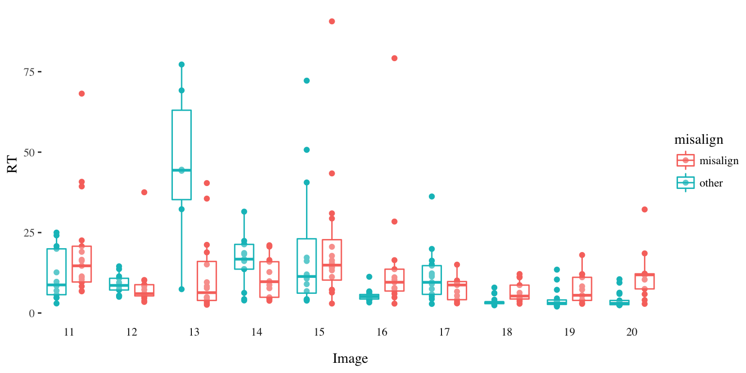
Distribution of Response Time per Image (Round 2)
Analysis
Linear Models
The easiest way to seperate between an image effect and a subject effect is to run a simple linear model with both factors, which is what we do below.
Let’s just try to apply our coefficients method to the whole dataset and see what we get.
getCBCoef <- function(d, s, t) {
  dat <- d %>%
    filter(subNum %in% s & misalign==t) %>%
    mutate(
      subNum = as.factor(subNum)
      )
  m1 <- lm(RT ~ subNum + image,
          data=dat,
          contrasts=list(subNum="contr.Sum", image="contr.Sum")
        )
  coefs <- summary(m1)$coef[,1]
  coefs <- coefs[grep("subNum", names(coefs))]
  nums <- gsub("[^0-9]*", "", names(coefs))
  df <- data.frame(
    nums = nums,
    coef = coefs
    )
  names(df)[2] <- paste("coef", t, sep="_")
  df
}
getPreCoef <- function(d, s, t) {
  dat <- d %>%
    filter(subNum %in% s & type==t) %>%
    mutate(
      subNum = as.factor(subNum)
      )
  m1 <- lm(Rating ~ subNum + imgNum,
          data=dat,
          contrasts=list(subNum="contr.Sum", imgNum="contr.Sum")
        )
  coefs <- summary(m1)$coef[,1]
  coefs <- coefs[grep("subNum", names(coefs))]
  nums <- gsub("[^0-9]*", "", names(coefs))
  df <- data.frame(
    nums = nums,
    coef = coefs
    )
  names(df)[2] <- paste("coef", t, sep="_")
  df
}

# Let's restrict ourselves to sub1
grp <- sub1

cb.mis <- getCBCoef(cb, grp, "misalign")
cb.other <- getCBCoef(cb, grp, "other")

pre.o <- getPreCoef(pre.all, grp, "o")
pre.x <- getPreCoef(pre.all, grp, "x")
pre.f <- getPreCoef(pre.all, grp, "f")

all <- cb.mis %>%
  inner_join(cb.other, by="nums") %>%
  inner_join(pre.o, by="nums") %>%
  inner_join(pre.x, by="nums") %>%
  inner_join(pre.f, by="nums")

all$cb_diff <- all$coef_misalign - all$coef_other
all$pre_diff <- all$coef_o - all$coef_x

# pre.c1 <- getPreCoef(pre.all, grp, "c1")
# pre.c0 <- getPreCoef(pre.all, grp, "c0")gpairs(data.frame(all[,-1]))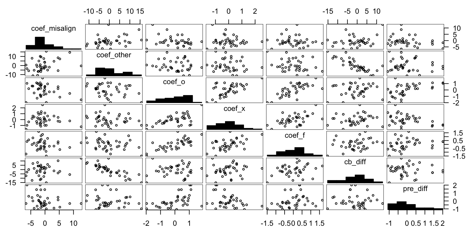
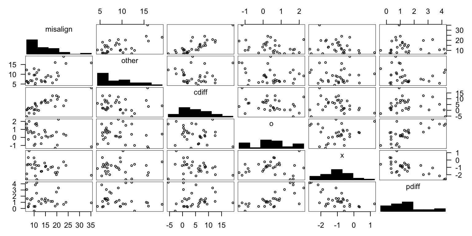
Averaging
Here’s another method:
# well this didn't work
cbs <- cb %>%
  filter(subNum %in% sub2) %>%
  group_by(subNum, misalign) %>%
  summarise(med_rt=mean(RT)) %>%
  spread(misalign, med_rt) %>%
  mutate(cdiff = misalign - other)
cbs %>% head| subNum | misalign | other | cdiff |
|---|---|---|---|
| 1 | 6.96120 | 6.2010 | 0.760200 |
| 3 | 16.10960 | 9.3527 | 6.756900 |
| 5 | 13.35823 | 6.1964 | 7.161831 |
| 7 | 15.15080 | 8.4894 | 6.661400 |
| 9 | 20.23030 | 10.7860 | 9.444300 |
| 13 | 24.02690 | 15.5142 | 8.512700 |
pres <- pre.all %>%
  filter(subNum %in% sub2 & type %in% c("o", "x")) %>%
  group_by(subNum, type) %>%
  summarise(avg_rat=mean(Rating)) %>%
  spread(type, avg_rat) %>%
  mutate(pdiff = o - x)
pres %>% head| subNum | o | x | pdiff |
|---|---|---|---|
| 1 | 0.9166667 | -0.6666667 | 1.5833333 |
| 3 | 0.0370370 | -1.2962963 | 1.3333333 |
| 5 | -0.0256410 | -1.5384615 | 1.5128205 |
| 7 | 0.1666667 | -0.8333333 | 1.0000000 |
| 9 | -0.9583333 | -1.6666667 | 0.7083333 |
| 13 | 0.2592593 | -0.7407407 | 1.0000000 |
pall <- cbs %>% inner_join(pres)gpairs(data.frame(pall[,-1]))