Taste Prediction
Introduction
What if you could tell a person’s taste typicality just from their resting state brain scans? In a previous post, we formulated a measure of a person’s taste typicality, using some fancy Euclidean distance metric. Now, we can match that measurement to the individual’s resting state, which is something like a correlation (matrix) between the activity of different regions of the brain. It will be more convenient to talk about the resting state as a graph, where the nodes are the regions of the brain, and the edge weights correspond to the correlation.
We expect that there are certain regions of the brain whose behaviour correlate strongly with the trait in question (either negative or positively). How do we go about testing this though?
The current method is as follows: for each edge of the correlation graph, run a robust regression between the vector of weights and the trait, and note the sign of the coefficient and the \(p\)-value. Then, by thresholding at some significance level (\(p < 0.01\)), we have a set of edges that strongly (positively) correlate with the target trait. We can then sum the weights of the positive edge set to produce a measure of positive network strength for each individual1 The reason put forward for this aggregation is that it is a more robust measure, versus just looking at individual ones..
It is clear that this method will pick up spurious correlations, as it is actively searching for them. Below we see what happens when we generate random noise for both the reference vector and the correlation matrix, and perform the method.
library(robustbase)
library(quantreg)
set.seed(99)
n <- 25
p <- 100
t <- rnorm(n) # for taste
s <- array(,c(n,p,p))
# actually sample a random correlation matrix
q <- 25
for (i in 1:n) {
  # guessing this is what they mean by Fisher-normalized?
  s[i,,] <- scale(cor(matrix(rnorm(q*p), ncol=p)))
}
# previously: just made it random noise
# s <- array(rnorm(n*p*p), c(n,p,p)) # for scans
# # symmetrizing
# for (i in 1:n) {
#   s[i,,][lower.tri(s[i,,])] <- t(s[i,,])[lower.tri(s[i,,])]
# }
cors <- matrix(,nrow=p, ncol=p)
pvas <- matrix(,nrow=p, ncol=p)
combs <- combn(1:p, 2)
for (col in 1:ncol(combs)) {
i <- combs[1,col]
j <- combs[2,col]
cfs <- coefficients(summary(rq(t ~ s[,i,j]), se="nid"))
pvas[i,j] <- cfs[2,4]
cors[i,j] <- cfs[2,1]
}
# positive/negative masks
pos <- (cors > 0) & (pvas < 0.01) & upper.tri(cors)
neg <- (cors < 0) & (pvas < 0.01) & upper.tri(cors)
pos.strength <- vector(,n)
neg.strength <- vector(,n)
for (i in 1:n) {
pos.strength[i] <- sum(s[i,,][which(pos)])
neg.strength[i] <- sum(s[i,,][which(neg)])
}Naturally, we see (below) that there is a positive (negative) correlation between taste and network strength.
plot(pos.strength, t)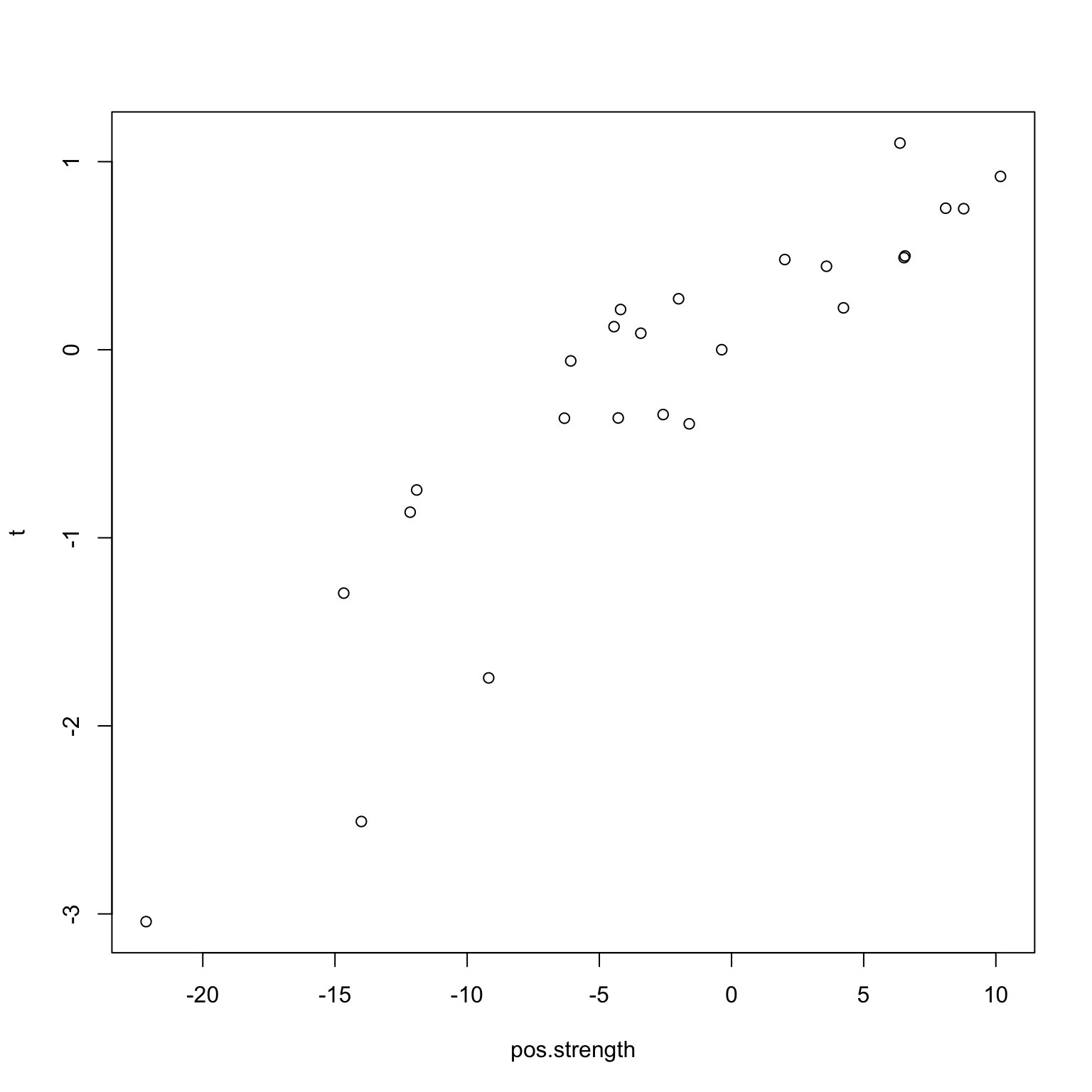
plot(neg.strength, t)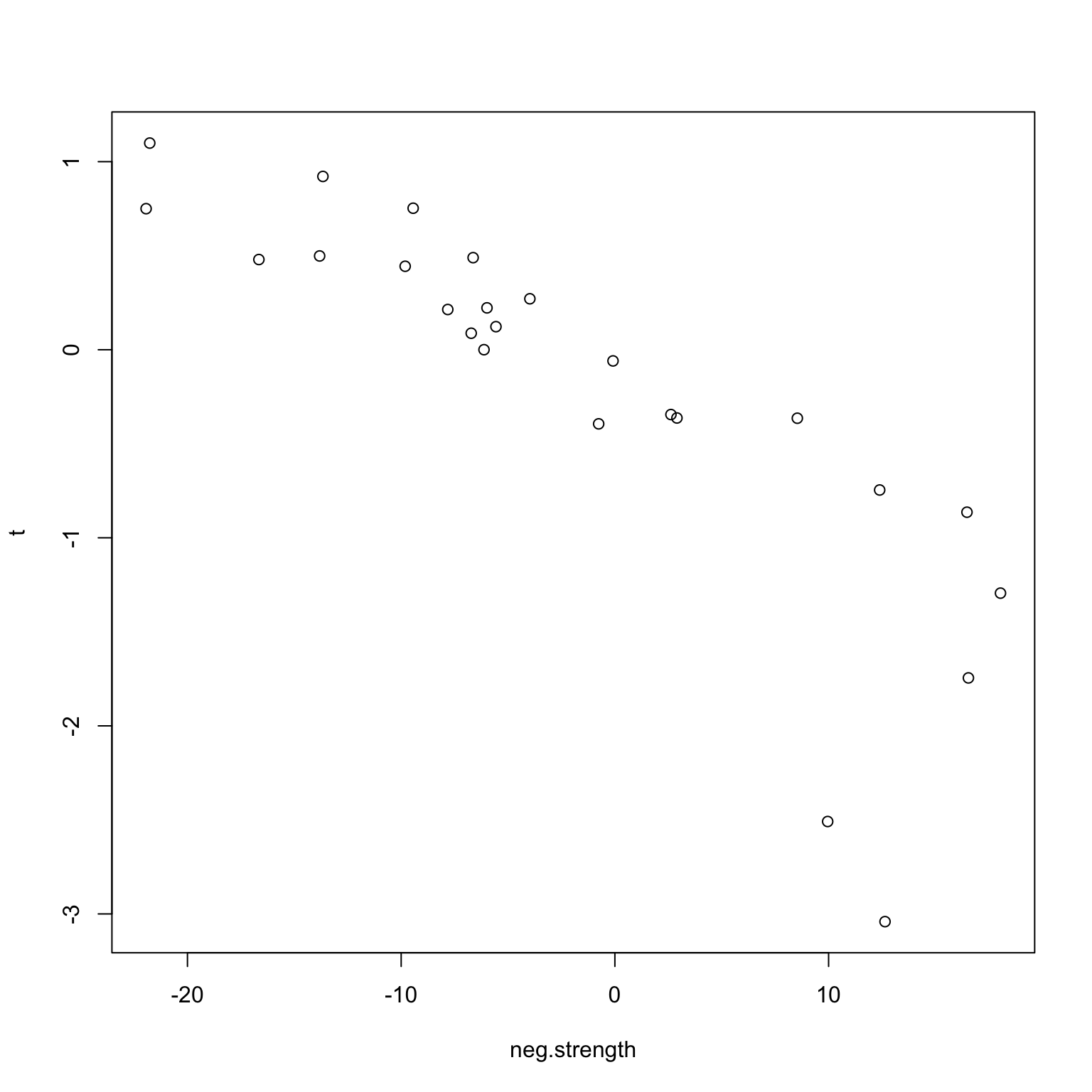
Validation
In order to check that the results are not spurious, we can perform a leave-one-out validation. Let’s first describe this procedure. Essentially, we leave an individual (\(k\)) out of the dataset and perform the same analysis on the remaining \(n-1\) individuals. This then generates a new positive edge set, and consequently a new positive network strength value for all individuals. We then build a model using the \(n-1\) positive network strength values and the corresponding taste value, and predict the individual \(k\)’s taste from his positive network strength.
The first issue I imagined was that leaving a single individual out should not greatly affect things, and in particular, because a robust method was chosen, the coefficients and \(p\)-values should not change much. Suppose in fact the positive edge sets did not change at all – in other words, we used a (hypothetical) robust regression whose results are invariant under leave-one-out. Then, we would get back this diagram when performing the validation on random noise, where we know that the correlations are simply spurious.
plot(predict(lm(t ~ pos.strength)), t)
abline(0,1)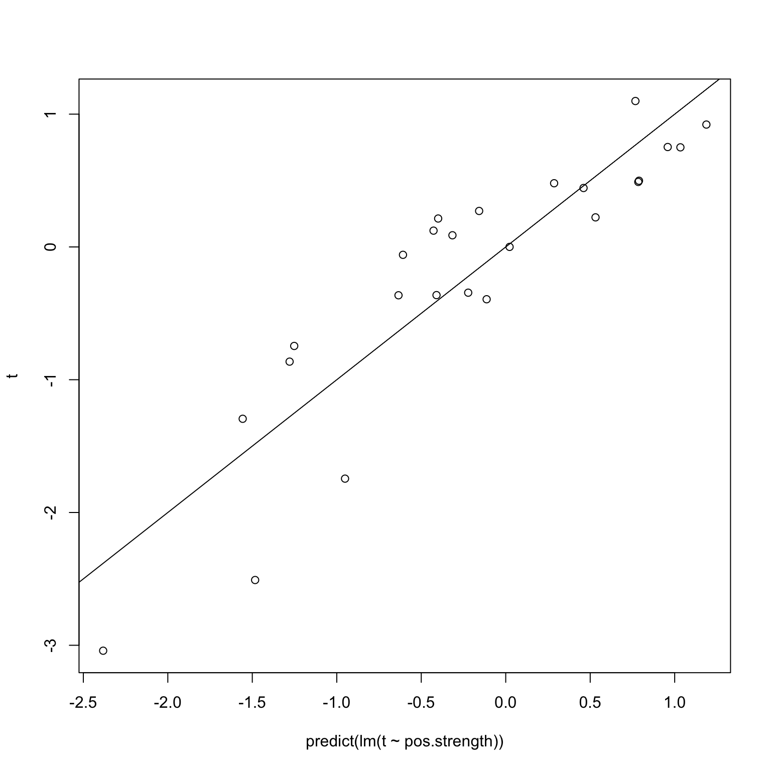
plot(predict(lm(t ~ neg.strength)), t)
abline(0,1)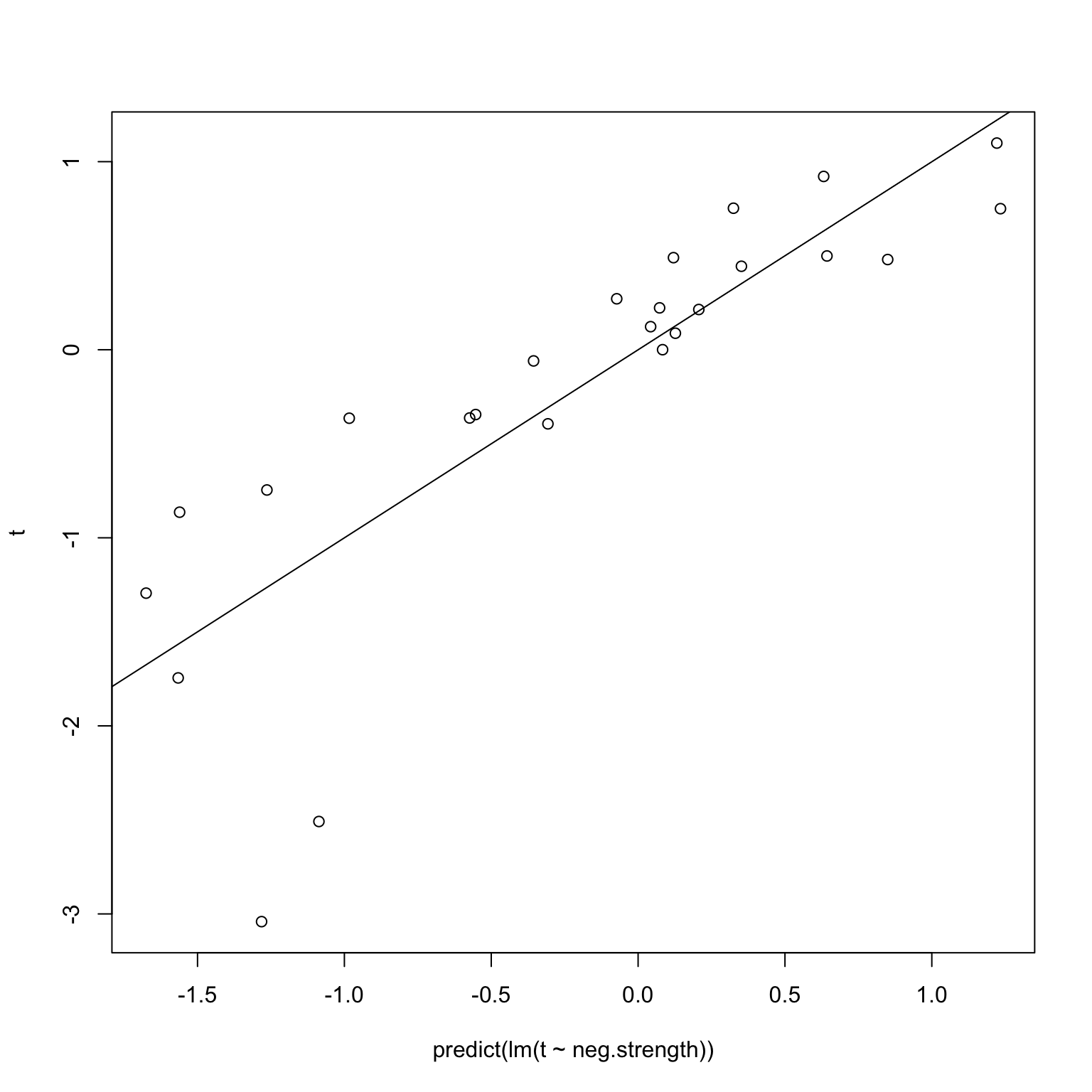
When using standard robust regressions like quantile regression, however, the coefficients and \(p\)-values can actually change quite a bit, especially at the \(p = 0.01\) range. I for one was surprised by how much. For instance, consider the random set of points below. How different is the \(p\)-value going to be between the whole set of points, and only the black points?
plot(t, s[,1,2], col=c(2, rep(1, n-1)))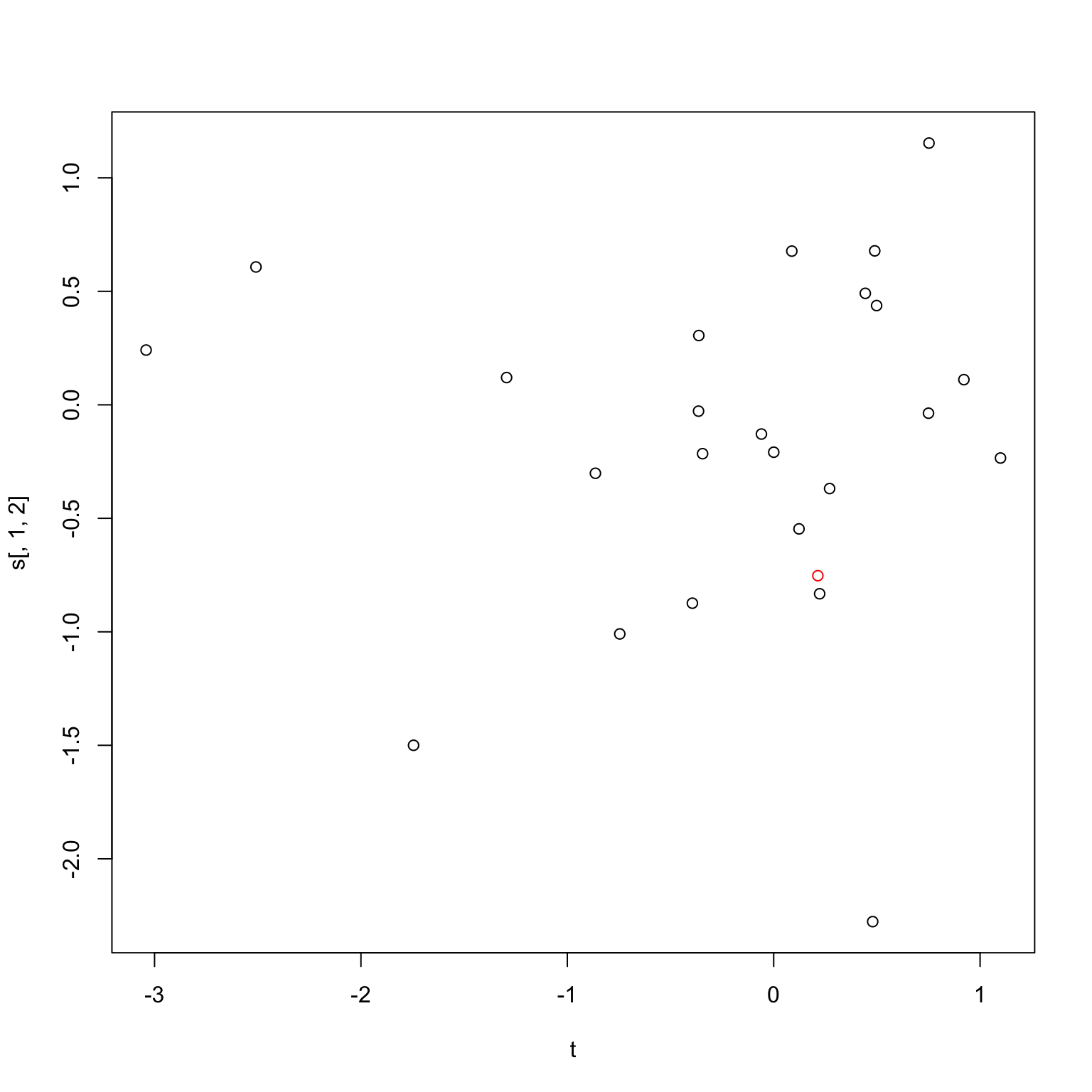
coefficients(summary(rq(t ~ s[,1,2]), se="nid"))| Value | Std. Error | t value | Pr(>|t|) | |
|---|---|---|---|---|
| (Intercept) | 0.0208916 | 0.3042777 | 0.0686595 | 0.9458541 |
| s[, 1, 2] | 0.0988371 | 0.2529699 | 0.3907070 | 0.6996093 |
coefficients(summary(rq(t[-1] ~ s[-1,1,2]), se="nid"))| Value | Std. Error | t value | Pr(>|t|) | |
|---|---|---|---|---|
| (Intercept) | 0.1002471 | 0.3042456 | 0.3294942 | 0.7448987 |
| s[-1, 1, 2] | 0.5655997 | 0.2486281 | 2.2748823 | 0.0330124 |
As it turns out, a considerable amount (\(p\)-value of 0.7 for the full set against a \(p\)-value of 0.03 for the one with just the red point removed). So the first question is, what exactly is accomplished by using the robust version of linear regression? I imagine the idea is that we want to do some sort of analysis that is robust to potential outliers, but since robust regression is generally more complicated and obscure that ordinary least squares, and our validation step involves removing points, we need to be careful about how our choice of a linear model interacts with the validation step.
What I find really weird about the whole set up is that we specifically pick edges that we have shown to be significant. Taking things to the extreme again, suppose we instead require that the significance level is at \(10^{-5}\), then I would expect that this would mean that the leave-one-out validation would make very little difference, since if the original plot is that significant, then leaving any one out should not change things.
So in some ways, this feels like an elaborate balancing act to me. We need to pick an appropriate \(p\)-value that isn’t too small or too large; we need to pick a linear model that isn’t too robust, nor too sensitive.
Let me make one final point regarding the high-level interpretation of what is going on. Essentially, the heuristic behind this leave-one-out method is that we are essentially simulating what would happen if we only saw those \(n-1\) individuals, and how our predictions would be on the \(n\)-th individual given the model constructed on the \(n-1\) individuals. This all sounds good, but the trouble arises from the fact that we do this \(n\) times, on almost the same dataset.
Simulations
# pb <- txtProgressBar(1, n, style=3)
t.pred <- vector(,n)
for (k in 1:n) {
  # setTxtProgressBar(pb, k)
  cors.k <- matrix(,nrow=p, ncol=p)
  pvas.k <- matrix(,nrow=p, ncol=p)
  combs <- combn(1:p,2)
  for (col in 1:ncol(combs)) {
    i <- combs[1,col]
    j <- combs[2,col]
    cfs <- coefficients(summary(rq(t[-k] ~ s[-k,i,j]), se="nid"))
    pvas.k[i,j] <- cfs[2,4]
    cors.k[i,j] <- cfs[2,1]
  }
  # positive/negative masks
  pos.k <- (cors.k > 0) & (pvas.k < 0.01) & upper.tri(cors.k)
  neg.k <- (cors.k < 0) & (pvas.k < 0.01) & upper.tri(cors.k)

  pos.k.strength <- vector(,n)
  neg.k.strength <- vector(,n)
  for (i in (1:n)) {
    pos.k.strength[i] <- sum(s[i,,][which(pos.k)])
    neg.k.strength[i] <- sum(s[i,,][which(neg.k)])
  }
  # now let's predict k's strength
  y <- t[-k]
  x <- pos.k.strength[-k]
  lm <- lm(y ~ x)
  t.pred[k] <- predict(lm, data.frame(x=pos.k.strength[k]))
  # what if we don't leave it out?
  # t.pred.noleave <- predict(lm(t ~ pos.k.strength), data.frame(pos.k.strength=pos.k.strength[k]))
}plot(t, t.pred)
abline(0,1)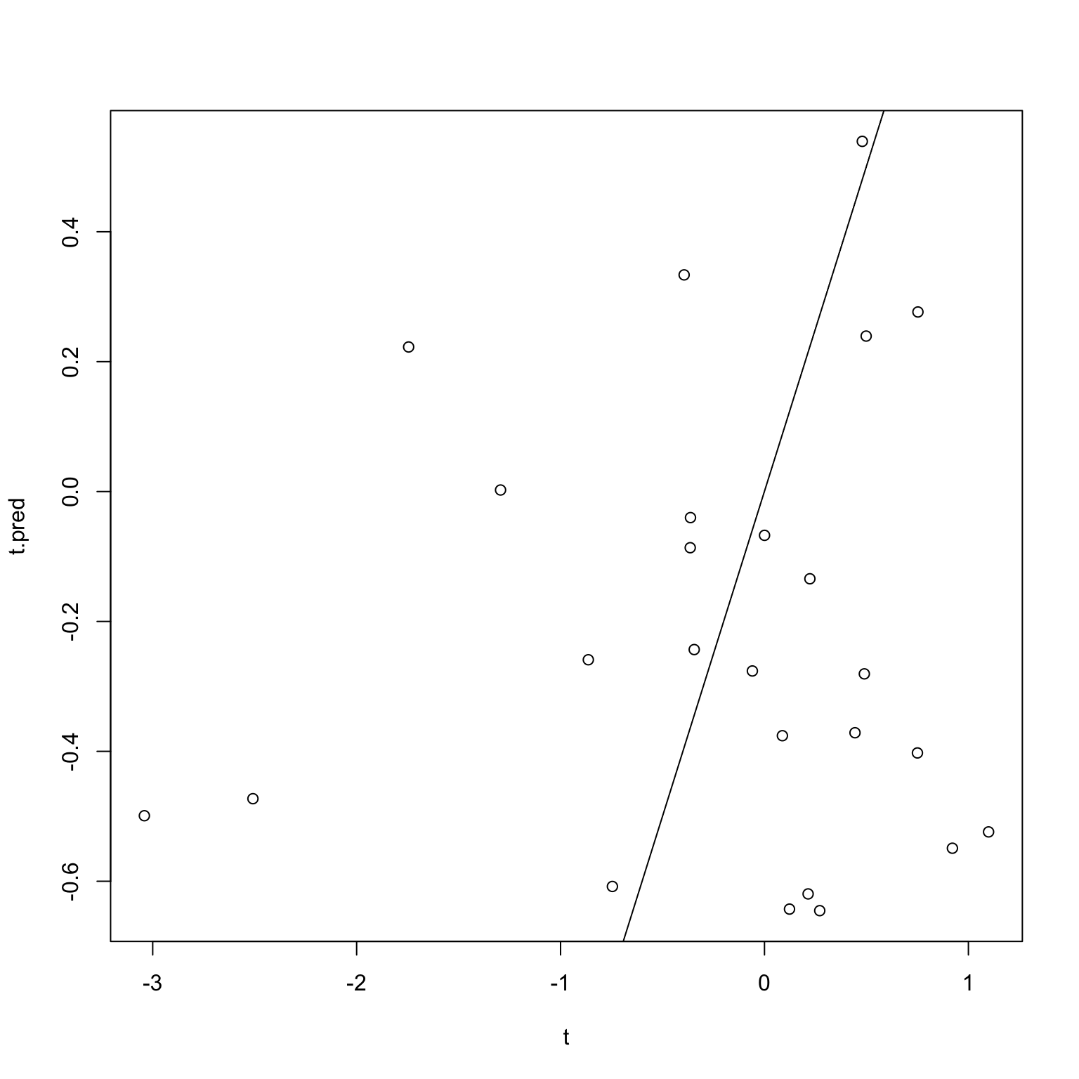
cor.test(t, t.pred)
    Pearson's product-moment correlation

data:  t and t.pred
t = 0.15915, df = 23, p-value = 0.8749
alternative hypothesis: true correlation is not equal to 0
95 percent confidence interval:
 -0.3667710  0.4227571
sample estimates:
       cor
0.03316645
Solution?
So now the question is, how do we do this rigorously? My first thought is that we need to perform some multiple testing correction here.