Homophily and Ranking

Social network generative models have reached an impasse. All the famous models take a very simple mechanism, and demonstrate that the repercussions produce networks that follow a documented feature of real-life social networks. But they only ever match one feature: small world, small diameter by random ties; preferential attachment, power law degree distribution.

What if homophily, together with the randomness of human personality/trait, is the driving force for what we see? Let’s find out!

Homophily

Let us model individuals as a vector of \(p\) Gaussian random variables that correspond to different vectors of characteristics. The size of \(p\) shall vary, as it may be the case that the magnitude of \(p\) drives some of the emergent behaviour11 For instance, one could claim that as civilization progresses, you have more characteristics to compare, which might then explain differences between rural and modern social networks.. For now, we have chosen the Gaussian distribution for simplicity.

The general idea is that vectors that are close in some metric should be friends. This is not new – objects such as the \(k\)-nearest neighbour graph or the \(\epsilon\)-neighbour graph have been studied. However, it seems that they haven’t been used to model human to human interactions, but rather generate similarity graphs of other kinds of entities. Perhaps a different perspective will produce something novel. The biggest problem is deciding what is the bare minimum complexity needed in order to elicit interesting results – after all, the social world is a messy place with a multitude of factors contributing in all directions.

For instance, there is the constraint of spacial separation. In the current model, we assume that as long as two people are similar enough, they will become friends, but this is obviously not realistic, as they might be on opposite ends of the world? But at the same time, in today’s society your location is not so much a hindrance with the power of the internet. What about cognitive load – we have a cap on the number of friends we can have?

What metric should we use? Should it be a proper metric that is symmetric? The problem with that is that we know proper social networks are directed.

Another crucial question is whether or not we model the network in a dynamic fashion or a static one. This poses a tradeoff between the simplicity of theoretical analysis on one side and the potential complexity of the resulting network on the other side.

A part of the motivation for this project is that there doesn’t seem to be any sort of framework whereby you can tweak parameters to produce a variety of social networks, and so this is an attempt to fill in that gap, hopefully.

Model Specification

Suppose we have \(n\) individuals with characteristic \(X_i \in \mathbb{R}^{p}\). The first simple idea is that every individual has a basis that describes their preferences towards people’s characteristics, which we model as a normalized Gaussian vector in \(\mathbb{R}^{p}\).

set.seed(0)
library(igraph)
library(ggraph)
# igraph_options(
#   vertex.label=NA,
#   vertex.size=2,
#   vertex.color="white",
#   edge.width=2,
#   arrow.size=0.5
#   )

ones <- function(n) matrix(1, nrow=n, ncol=1)

n <- 20 # number of individuals
p <- 40 # number of characteristics
m <- 8 # total number of friends

X <- matrix(rnorm(n*p), nrow=n)
w <- matrix(rnorm(n*p), nrow=n)
# normalizing
w <- t(apply(w, 1, function(x) x/sqrt(sum(x^2))))
stopifnot(sum(w[1,]^2) == 1)

The second is that different individuals will have varying thresholds for compatibility. Two implementations come to mind: a random number designating the threshold, or the threshold corresponding to a rank of compatibility scores (which corresponds to have a fixed number of friends).

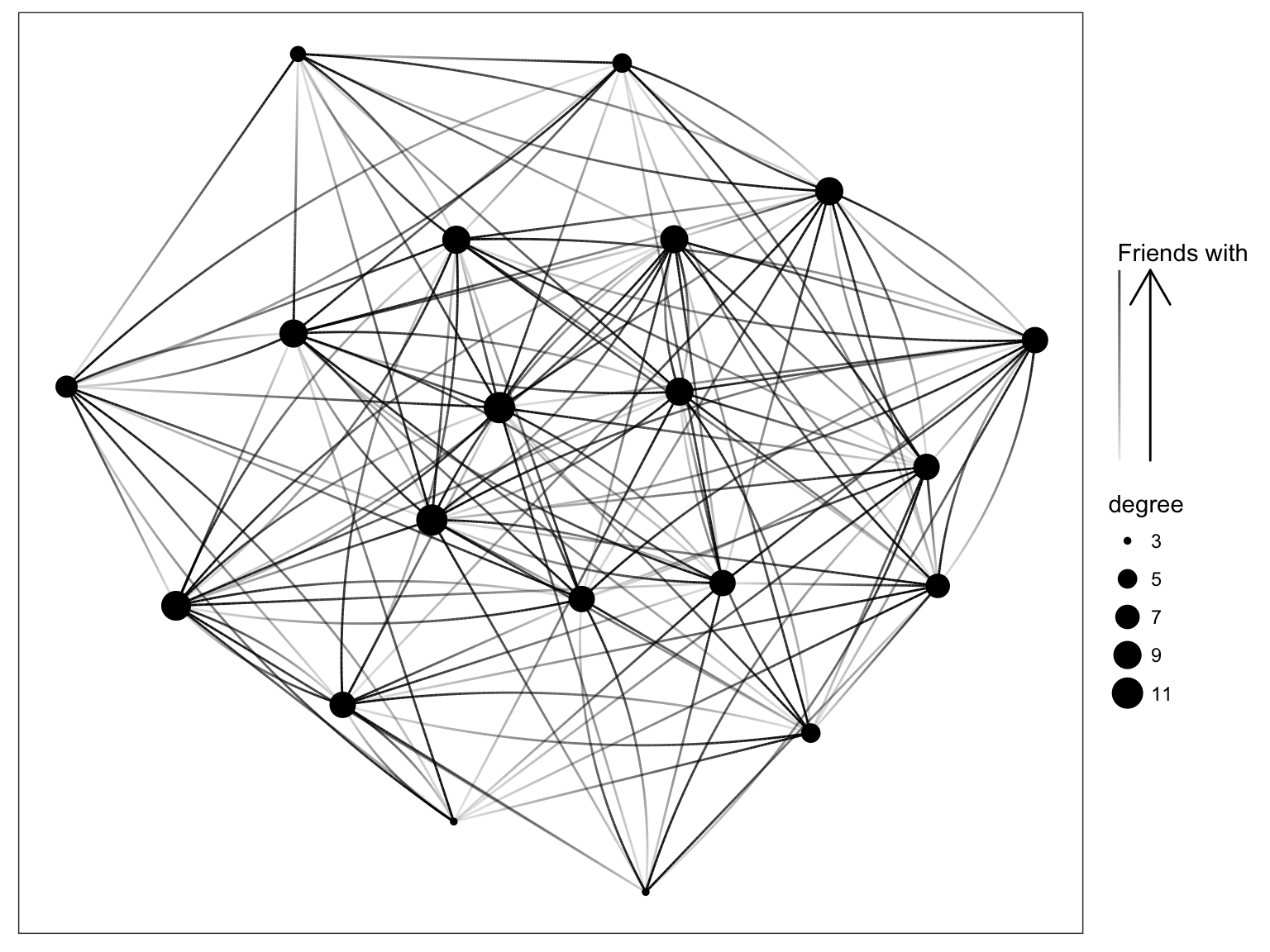
s <- runif(n, 2, 2)
Z <- matrix(, nrow=n, ncol=n)
for (i in 1:n) {
  dist <- mahalanobis(X, X[i,], diag(w[i,]^2))
  # RBF
  dist <- exp(-dist)
  Z[i,] <- (dist <= s[i])*1
}

g <- graph_from_adjacency_matrix(Z, diag=FALSE)
V(g)$degree <- degree(g, mode="in")
ggraph(g, 'igraph', algorithm = 'kk') + 
  geom_edge_fan(aes(alpha = ..index..)) + 
  geom_node_point(aes(size = degree)) +
  scale_edge_alpha('Friends with', guide = 'edge_direction') + 
  ggforce::theme_no_axes()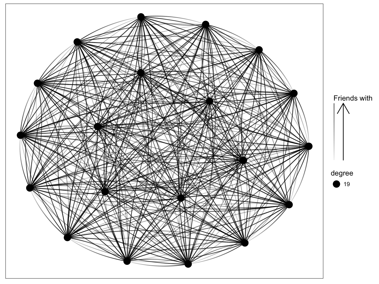

Z <- matrix(, nrow=n, ncol=n)
for (i in 1:n) {
  dist <- mahalanobis(X, X[i,], diag(w[i,]))
  top <- order(dist,decreasing=TRUE)[1:m]
  dist[top] <- 1
  dist[-top] <- 0
  Z[i,] <- dist
}

g <- graph_from_adjacency_matrix(Z, diag=FALSE)
V(g)$degree <- degree(g, mode="in")
ggraph(g, 'igraph', algorithm = 'kk') + 
  geom_edge_fan(aes(alpha = ..index..)) + 
  geom_node_point(aes(size = degree)) +
  scale_edge_alpha('Friends with', guide = 'edge_direction') + 
  ggforce::theme_no_axes()