Fundamental Limits of Estimating Parameters in a Stochastic Blockmodel

Simulations

Here we are checking to see how the estimate \[ \begin{align} \hat{p} = \frac{\sum_{ijk} B_{ijk}}{\rho_n \sum_{ij} A_{ij}} \end{align} \] fares in simulations.

library(igraph)
library(Matrix)
Nsim <- 10^3
res <- vector(,Nsim)
pp <- 0.4
p <- 0.4
n <- 10^5
rho <- sqrt(log(n))/n
N.all <- rbinom(Nsim, n, pp)
# pb <- txtProgressBar(min = 0, max = Nsim, initial = 0) 
for (i in 1:Nsim) {
  N <- N.all[i]
  c.sizes <- c(N, n-N)
  p.mat <- matrix(c(p*rho,0,0,0), nrow=2)

  g <- sample_sbm(n, p.mat, c.sizes, directed = FALSE, loops = FALSE)
  A <- as_adjacency_matrix(g, type="both", sparse=TRUE)

  sum.A <- sum(A)
  A2 <- A%*%A
  sum.B <- sum(A2) - sum(diag(A2))

  p.hat <- sum.B^2/(sum.A^3*rho)
  res[i] <- p.hat
  # setTxtProgressBar(pb,i)
}
hist(res)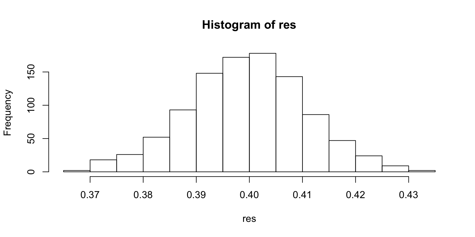

var(res)

[1] 0.0001251491

# sanity checking
# n <- 10
# p.mat <- matrix(c(1,1,1,1), nrow=2)
# c.sizes <- c(10,0)
# g <- sample_sbm(n, p.mat, c.sizes, directed = FALSE, loops = FALSE)
# A <- as_adjacency_matrix(g, type="both", sparse=TRUE)

Let’s turn it into a routine and see what happens when we change \(n\) and \(\rho_n\).

Nsim <- 10^2
pp <- 0.45
p <- 0.7
df <- data.frame(n=numeric(), r=numeric(), v=numeric())
for (nt in c("10^3", "10^4", "10^5")) {
  for (r in c("1", "sqrt(log(n))", "log(sqrt(n))", "log(n)")) {
    n <- eval(parse(text=nt))
    rho <- eval(parse(text=r))/n
    N.all <- rbinom(Nsim, n, pp)
    res <- vector(,Nsim)
    for (i in 1:Nsim) {
      N <- N.all[i]
      c.sizes <- c(N, n-N)
      p.mat <- matrix(c(p*rho,0,0,0), nrow=2)

      g <- sample_sbm(n, p.mat, c.sizes, directed = FALSE, loops = FALSE)
      A <- as_adjacency_matrix(g, type="both", sparse=TRUE)

      sum.A <- sum(A)
      A2 <- A%*%A
      sum.B <- sum(A2) - sum(diag(A2))

      p.hat <- sum.B^2/(sum.A^3*rho)
      res[i] <- p.hat
    }
    df <- rbind(df, data.frame(n=nt, r=r, v=var(res)))
  }
}
xtabs(1/v~n+r, data=df)

n/r	1	sqrt(log(n))	log(sqrt(n))	log(n)
10^3	10.29915	78.17433	113.9508	346.7706
10^4	140.85548	810.61940	2052.9501	5366.9762
10^5	1050.77507	9096.68515	24475.4677	98919.6015

library(ggplot2)
library(tidyr)
Nsim <- 10^2
pp <- 0.45
p <- 0.7
df <- data.frame(n=numeric(), r=numeric(), v=numeric())
for (nt in c("10^3", "10^4", "2*10^4", "5*10^4", "10^5")) {
  for (r in c("1", "sqrt(log(n))", "log(n)")) {
    n <- eval(parse(text=nt))
    rho <- eval(parse(text=r))/n
    N.all <- rbinom(Nsim, n, pp)
    res <- vector(,Nsim)
    for (i in 1:Nsim) {
      N <- N.all[i]
      c.sizes <- c(N, n-N)
      p.mat <- matrix(c(p*rho,0,0,0), nrow=2)

      g <- sample_sbm(n, p.mat, c.sizes, directed = FALSE, loops = FALSE)
      A <- as_adjacency_matrix(g, type="both", sparse=TRUE)

      sum.A <- sum(A)
      A2 <- A%*%A
      sum.B <- sum(A2) - sum(diag(A2))

      p.hat <- sum.B^2/(sum.A^3*rho)
      res[i] <- p.hat
    }
    df <- rbind(df, data.frame(n=nt, r=r, v=var(res)))
  }
}

new.df <- df
new.df$n <- apply(new.df, 1, function(x) eval(parse(text=x[1])))
new.df$n2.rho <- apply(new.df, 1, function(x) {
  n <- as.integer(x[1])
  rho <- eval(parse(text=x[2]))
  1/(n^2*rho)
})
new.df$n.rho <- apply(new.df, 1, function(x) {
  n <- as.integer(x[1])
  rho <- eval(parse(text=x[2]))
  1/(n*rho)
})
new.df$n.n <- apply(new.df, 1, function(x) {
  n <- as.integer(x[1])
  rho <- eval(parse(text=x[2]))
  1/(n)
})
new.df$n.rho2 <- apply(new.df, 1, function(x) {
  n <- as.integer(x[1])
  rho <- eval(parse(text=x[2]))
  1/(n*rho^2)
})
df2 <- gather(new.df, type, value, v:n.rho2)
ggplot(df2, aes(x=n, y=1/value, group=type, color=type)) + geom_point() + geom_line() + facet_grid(.~r) + scale_y_log10() + scale_x_log10() + theme_minimal()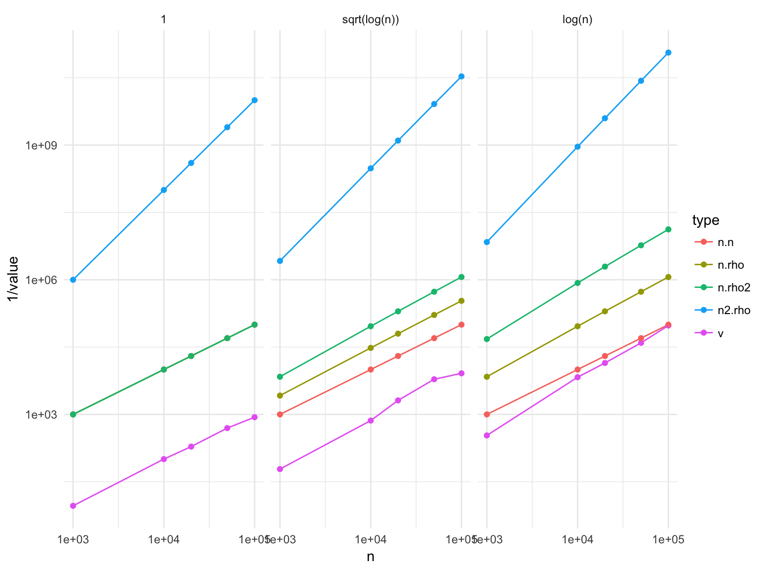

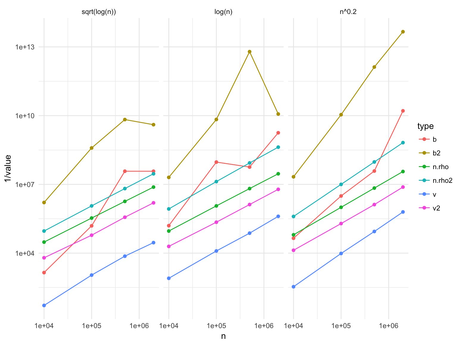
Nsim <- 10^3
pp <- 0.2
p <- 0.1
df <- data.frame(n=numeric(), r=numeric(), v=numeric(), b=numeric(), v2=numeric(), b2=numeric())
for (nt in c("10^4", "10^5", "5*10^5", "2*10^6")) {
  for (r in c("sqrt(log(n))", "log(n)", "n^0.2")) {
    n <- eval(parse(text=nt))
    rho <- eval(parse(text=r))/n
    N.all <- rbinom(Nsim, n, pp)
    res <- vector(,Nsim)
    res2 <- vector(,Nsim)
    for (i in 1:Nsim) {
      N <- N.all[i]
      g <- sample_gnp(N, p*rho)
      A <- as_adjacency_matrix(g, type="both", sparse=TRUE)

      sum.A <- sum(A)
      A2 <- A%*%A
      sum.B <- sum(A2) - sum(diag(A2))

      p.hat <- sum.B^2/(sum.A^3*rho)
      res[i] <- p.hat
      res2[i] <- sum.A/N^2/rho
    }
    df <- rbind(df, data.frame(n=nt, r=r, v=var(res), b=mean(res-p)^2, v2=var(res2), b2=mean(res2-p)^2))
  }
}

new.df <- df
new.df$n <- apply(new.df, 1, function(x) eval(parse(text=x[1])))
new.df$n.rho <- apply(new.df, 1, function(x) {
  n <- as.integer(x[1])
  rho <- eval(parse(text=x[2]))
  1/(n*rho)
})
new.df$n.rho2 <- apply(new.df, 1, function(x) {
  n <- as.integer(x[1])
  rho <- eval(parse(text=x[2]))
  1/(n*rho^2)
})
df2 <- gather(new.df, type, value, v:n.rho2)
ggplot(df2, aes(x=n, y=1/value, group=type, color=type)) + geom_point() + geom_line() + facet_grid(.~r) + scale_y_log10() + scale_x_log10() + theme_minimal()